The 30–60-day Intraseasonal Variability of Sea Surface Temperature in the South China Sea during May–September
2018-03-07JiangyuMAOandMingWANG
Jiangyu MAOand Ming WANG
1LASG,Institute of Atmospheric Physics,Chinese Academy of Sciences,Beijing 100029,China
2University of Chinese Academy of Sciences,Beijing 100049,China
1.Introduction
Geographically,the South China Sea(SCS)is the largest marginal sea in the western North Pacific,situated at the center of the Asian–Australian monsoon region(Wang et al.,2009).Meteorologically,it is a key area where the subtropical East Asian monsoon subsystem interacts with the tropical South Asian monsoon,western North Pacific(WNP),and Australian monsoon subsystems(Chen and Chen,1995;Wang et al.,2009).Thus,the SCS monsoon belongs to an important tropical subsystem of the East Asian monsoon(Lau et al.,1988;Ding,1994;Zhou et al.,2005),with the SCS summer monsoon(SCSSM)dominated by southwesterlies,while northeasterlies prevail during boreal winter.The SCS also acts as a moisture pathway for water vapor transport from the Indian Ocean and western Pacific into eastern China in summer(Ding,1994;Ding and Chan,2005;Wang et al.,2009).Therefore,the SCSSM and its variability have tremendous impacts on local and regional weather and climate.
Within the annual cycle or within a particular season,intraseasonal oscillations(ISOs)are dominant components of monsoon variability in the Asian monsoon regime,characterized by active and break sequences with episodic fluctuations in rainfall intensity(Webster et al.,1998).The intraseasonal variability of the SCSSM has been found to be dominated by 30–60-day and 10–20-day ISOs(Mao and Chan,2005).The 30–60-day ISO of the SCSSM features a trough–ridge seesaw circulation pattern over the SCS in which an anomalous cyclone(anticyclone)together with enhanced(suppressed)convection propagates northward from the equator to the northern SCS.When such an anomalous cyclone(anticyclone)reaches the northern SCS,suppressed(enhanced)convection is simultaneously induced over the Yangtze Basin in centraleastern China,which indicates an intraseasonal interaction between the SCSSM and the extratropical East Asian summer(Chen et al.,2000;Mao and Chan,2005;Lu et al.,2014).The 10–20-day oscillation of the SCSSM manifests as the alternating occurrence of northwestward-migrating anomalous cyclones and anticyclones over the SCS that originate in the equatorial western Pacific(Mao and Chan,2005;Wu,2010).Similarly,when the anomalous cyclone(anticyclone)moves into the northern SCS,the anomalous northeasterlies(southwesterlies)on its northern side can lead directly to reduced(enhanced)rainfall over southern China,again suggesting the impact of the intraseasonal activities of the SCSSM on weather and climate anomalies over adjacent regions.
Air–sea interactions lead to significant intraseasonal variability of sea surface temperature(SST)in the SCS(Duvel and Vialard,2007;Roxy and Tanimoto,2012;Wu et al.,2015),as revealed by satellite data from the Tropical Rainfall Measuring Mission(TRMM)Microwave Imager(TMI)(Wentz et al.,2000).In investigating the influence of SST on the 30–60-day ISO of the SCSSM during April–July,Roxy and Tanimoto(2012)identified large standard deviations of the intraseasonal SST fluctuations of greater than 0.3°C at a period of 30–60 days in the central-western SCS,with the area-averaged SST being significantly correlated with local precipitation on the 30–60-day timescale.They suggested an ocean-to-atmosphere effect in the SCS,where positive SST anomalies tend to favor conditions for convective activity and sustain enhanced precipitation during the SCSSM.Conversely,increased cloudiness associated with precipitation would certainly cool the SST,leading to negative SST anomalies.This mechanism gives an intraseasonal atmospheric forcing of the underlying ocean.Thus,the formation of intraseasonal SST variations in the SCS is mostly attributed to changes in wind-related surface latent heat flux and cloud-related surface shortwave radiation flux(Roxy and Tanimoto,2012;Wu and Chen,2015).
Considering the seasonality and regionality of atmospheric ISOs,Wu et al.(2015)focused on the SCS and WNP regions to investigate the factors affecting intraseasonal SST variations in terms of surface heat flux and surface wind stress–related oceanic upwelling.Importantly,they compared the contributions in boreal summer(May to September)and boreal winter(November to the following March)of different processes influencing the intraseasonal SST fluctuations on both the 10–20-day and 30–60-day timescales.The intraseasonal SST variations are comparable on the 10–20-day and 30–60-day timescales but larger during summer than during winter,with a clear difference in the distribution of the local correlation of the SST tendency with net surface heat flux(NSHF)and surface wind speed between the 10–20-day and 30–60-day time scales during summer.This different summer response indicates that the structure of atmospheric ISOs is important for determining the distribution of intraseasonal SST variability and the atmosphere-to-ocean impact in the SCS and WNP areas.Actually,some previous studies have noted both the impact of intraseasonal SST variations on the propagation of atmospheric ISOs and their coupling in tropical oceans(Woolnough et al.,2000;Fu et al.,2003;Bellon et al.,2008;Wu et al.,2008;Chou and Hsueh,2010;Roxy et al.,2013).
Apart from atmospheric thermodynamic forcing associated with surface heat fluxes,oceanic dynamics including horizontal advection and vertical entrainment in the upper ocean can also lead to variations of SST(e.g.,Duvel and Vialard,2007;Bellon et al.,2008).As suggested by Qu(2003),the vertical entrainment is another dominant term that cools the SST in the NWP,since the horizontal temperature gradient is usually weak within the upper ocean mixed layer,so the horizontal temperature advection by the mixedlayer currents is negligible.However,the relative contribution of subsurface water entrainment to the SST cooling may be different in different basins and different seasons(Duvel and Vialard,2007;Chou and Hsueh,2010).In exploring the causes of the strong intraseasonal SST perturbations of more than 1.5°C over a large region in the Indian Ocean between 5°and 10°S during winter 1999,Harrison and Vecchi(2001)suggested that the strong SST variations are mainly due to vertical entrainment because the thermocline is closer to the surface in the winter season.Chou and Hsueh(2010)suggested that,during summer,intraseasonal SST variations are dominated by surface-wind-induced forcing,latent heat flux,and subsurface water entrainment via changes of the mixedlayer depth in the WNP,but they did not provide direct evidence for changes in vertical entrainment.For the SCS,based on local correlations of the SST tendency with NSHF and wind speed,Wu et al.(2015)argued that,in summer,the intraseasonal SST perturbations in the northern SCS are related to surface heat flux,entrainment,and upwelling,while those in the southern SCS are mainly related to surface heat flux and entrainment.However,this relative importance of the entrainment in the SCS is inferred from surface wind information alone,as the effects of entrainment and upwelling are respectively proportional to the surface wind speed and wind stress curl.
Note that Roxy and Tanimoto(2012)examined the intraseasonal behavior of the SCSSM forced by SST anomalies only for the period April–July.However,the climatological SCSSM onset occurs around the fourth pentad of May(Mao et al.,2004;Zhou et al.,2005),so the period April–July studied by Roxy and Tanimoto(2012)consists of the winter monsoon to summer monsoon transition months of April and May and the early summer months of June and July.The SCSSM prevails throughout the entire boreal summer from May to September,although it is sometimes affected to some extent by typhoons after August.As the intraseasonal standard deviation of SST in the SCS is larger on the 30–60-day time scale than on the 10–20-day time scale(Wu et al.,2015),it is necessary to understand how the strong 30–60-day intraseasonal SST variability is generated in the SCS during summer.Note also that Wu et al.(2015)only qualitatively analyzed the surface wind stress curl–related oceanic upwelling and surface wind speed–related entrainment;the oceanic upwelling and entrainment were simply estimated from the surface wind stress and wind speed,respectively,rather than strictly calculated from the formulas in the thermodynamic equation for the mixed-layer temperature.
Therefore,the objective of this study is to characterize the 30–60-day intraseasonal SST variability in the SCS during the entire boreal summer(May–September)and to examine the physical mechanisms driving it(the thermodynamic forcing of atmospheric ISOs and oceanic dynamics responsible for upper-ocean vertical entrainment)by quantitatively diagnosing all components of the oceanic mixed-layer temperature equation.This will provide an understanding of the generation of the intraseasonal SST perturbations in the SCS and their feedback on atmospheric ISOs,as well as the consequent anomalous weather and climate both locally and regionally.
2.Data and methods
2.1.Data
Daily TRMM satellite-based TMI SST data(Wentz et al.,2000)are used in this study to identify the intraseasonal variability;the data are available since 1998 over the tropical–extratropical regions(38.5°S–38.5°N)with a high spatial resolution of 0.25°×0.25°.Duvel and Vialard(2007)compared the intraseasonal standard deviations of the SST in the 20–90-day band between the TMI SST dataset and the optimally interpolated SST(OISST)products(Reynolds and Smith,1994),and found that OISST notably underestimates the intraseasonal SST variability,especially in the equatorial Indian Ocean,while TMI SST performs better.This is because OISST is mostly based on measurements in the atmospheric infrared window,which is susceptible to cloud screening impairment of the sampling of the SST variability,while the TMI-measured SST is nearly free of cloud influence and is thus well-suited to the study of convection-related air–sea interaction(Duvel and Vialard,2007).Therefore,this study is mainly based on TMI SST data.To obtain daily TMI SST,both spatial filling and linear temporal interpolation are performed to reduce gaps in the data,with the spatial resolution decreasing to 1°×1°,as implemented by Wu et al.(2015).Finally,a three-day running mean is applied to produce the daily mean SST field for the period 1998–2013.
Relevant upper-ocean data, including temperature,mixed-layer depth,horizontal currents,and vertical velocity,are extracted from the NCEP’s Global Ocean Data Assimilation System(GODAS)oceanic reanalysis(Behringer and Xue,2004;Huang et al.,2010)for the period 1998–2013.The GODAS products have a 1°resolution in the zonal direction and a variable grid resolution in the meridional direction,with a 1/3°resolution between 10°S and 10°N.There are 40 levels in the vertical direction,with a 10-m resolution in the upper 200 m.We linearly interpolate the pentad GODAS data to generate daily values,following Wang et al.(2012).
Daily atmospheric circulation data,such as 10-m surface winds,are derived from the ECMWF’s interim reanalysis product(ERA-Interim)for the period 1998–2013,with a spatial resolution of approximately 80 km and 60 vertical levels from the surface up to 0.1 hPa(Berrisford et al.,2011).Also used are daily rainfall data from the Global Precipitation Climatology Project(GPCP)(Huffman et al.,2001;Xie et al.,2003)for the same period.
At the air–sea interface,the daily surface heat flux data in terms of shortwave radiation,longwave radiation,sensible heat and latent heat fluxes are extracted from the newly developed TropFlux products(Praveen Kumar et al.,2012,2013).TropFlux is available at a 1°×1°resolution over the entire 30°S–30°N region from 1989.The dataset is largely derived from a combination of ERA-Interim reanalysis data for turbulent and longwave radiation fluxes,and the International Satellite Cloud Climatology Project(ISCCP)for surface shortwave radiation flux,with all input products being bias-and amplitude-corrected on the basis of Global Tropical Moored Buoy Array data before surface net heat flux and wind stresses are computed using the COARE v3 bulk algorithm.A precise description of the flux computation procedure,as well as a detailed evaluation against other daily air–sea heat flux alternatives covering the same period(OAFLUX,NCEP,NCEP2,ERA-I)may be found in Praveen Kumar et al.(2012).
These multi-source atmospheric and oceanic datasets with different horizontal resolutions are all interpolated onto the same 1°×1°grid for this study.
2.2.Methods
The Lanczos bandpass filter(Duchon,1979)is a commonly used filtering technique to isolate intraseasonal components because of its ability to strongly reduce the Gibbs oscillation(e.g.,Kikuchi et al.,2012;Li and Zhou,2015).To identify the regional distributions of significant intraseasonal SST perturbations with different quasi-periodicities in the SCS during boreal summer,the Lanczos bandpass filter is applied to the daily SST anomaly time series at each grid point to extract dominant intraseasonal signals in the 10–90-day range.Note that the daily SST anomaly time series at each grid is calculated by removing the climatological annual cycle from the raw data.Such a filtering approach is also applied to other atmospheric and oceanic variables to obtain the corresponding intraseasonal components in the present study.
To verify the statistical significance of the specific periodicity of intraseasonal SST variability during boreal summer,especially for the 30–60-day timescale,we follow Wu et al.(2015)and apply power spectral analysis to the areaaveraged SST anomaly time series over the key region that has large intraseasonal standard deviation each summer.The mean power spectrum is then calculated as the average of the individual power spectra for the 16 summers from 1998 to 2013,thereby obtaining the common periodicity characteristics.The statistical significance of the power spectrum is tested based on the method of Gilman et al.(1963)for a rednoise process.
The local change of SST depends on atmospheric thermal forcing and oceanic dynamical processes.To explore their relative contributions to the formation of strong intraseasonal SST variability,we examine quantitatively the mixed-layer heat budget in the SCS,since the mixed-layer temperatureTmis a good proxy of SST under the assumption of vertically uniform mixed-layer temperature of depthhm.
As in Huang et al.(2010),the mixed-layer temperature equation can be expressed as
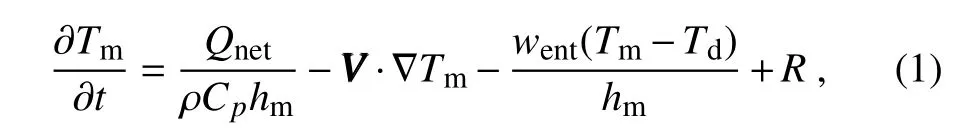
whereQnetis the net heat flux within the mixed-layer(abbreviated as MNHF),which is calculated asQnet=Q0−Qd.Q0is the downward NSHF(actually,the above-mentioned NSHF),consisting of shortwave radiation,longwave radiation,latent heat and sensible heat fluxes at the sea surface.Qdis the downward radiative heat flux across the base of the mixed-layer(actually,the penetrated solar radiation),and is calculated according to the empirical formula given by Paulson and Simpson(1977).Note thatQ0andQdare sometimes expressed explicitly in the mixed-layer heat budget equation(e.g.,Fu et al.,2003;Du et al.,2005)on the sea surface.VV Vdenotes the horizontal currents,wentis the entrainment rate,Tdis the water temperature below the base of the mixed-layer,ρ is the density of sea water,andCpis the specific heat capacity.Ris the residual term resulting from unresolved subgridscale turbulence.In the following,the term on the left-hand side of Eq.(1)is referred to as the SST tendency or the local rate of change of SST,and the first three terms on the righthand side as,from left to right,the thermal forcing associated with MNHF,horizontal advection,and vertical entrainment.In the present study,we utilize daily GODAS data to compute each of these terms to show the physical processes that control temperature changes in the mixed layer,demonstrating the relative roles of different processes in forcing the intraseasonal SST fluctuation in the SCS.The difference between the SST tendency and the sum of the first three terms on the righthand side is treated as the residual term to ensure closure of the mixed-layer heat budget.
To identify the spatial structure and temporal evolution of the intraseasonal SST variability in the SCS in relation to atmospheric thermodynamic forcing,we carry out composite analysis of strong intraseasonal SST events.The statistical significance of the composite anomalous variables is estimated using the Student’st-test.To detect the origin of an intraseasonal SST perturbation and its subsequent propagation associated with surface thermal forcing,we also calculate lead–lag correlations of area-averaged intraseasonal SST time series over the core region in the SCS with those of other variables,such as anomalous rainfall and NSHF,at each grid point.The statistical significance of the correlation coefficients is tested on the basis of two-tailed probabilities,in which the effective sample size of the intraseasonal anomaly time series for a particular variable is re-estimated using the method of Bretherton et al.(1999),since the time filtering described above may reduce the degrees of freedom of the intraseasonal anomaly time series.
3.Spatial and intraseasonal variations of SST in the SCS
3.1.Identification of the dominant 30–60-day SST variability
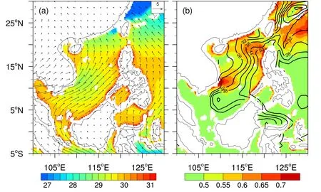
Fig.1.(a)Climatology of boreal summer(May–September)SST(shading;units:°C)and surface winds(vectors;units:m s−1)over the SCS for the period 1998–2013.The magnitude of the reference vector is given in the top-right corner of the figure.(b)Standard deviation(shading;units:°C)of the intraseasonal SST variability in the 10–90-day band and climatological boreal summer mixed-layer depth(contours;units:m)for the same period as(a).
Figure 1 shows the climatological distributions of TMI SST and mixed-layer depth in the SCS along with the surface winds in summer(May–September).Under the prevail-ing southwesterlies,the underlying mean SST is generally higher than 28.5°C(Fig.1a),which favors convective precipitation(Lau and Yang,1997).The corresponding mixed-layer depth exhibits an eastward increasing structure,with the shallowest depths(below 20 m)in the western SCS.The mixedlayer depth is mostly less than 50 m over the entire SCS(Fig.1b),which is much shallower than that during boreal winter shown in Wu et al.(2015).
As suggested by Duvel and Vialard(2007),the amplitude of intraseasonal SST variations is inversely proportional to the mixed-layer depth.We calculate the standard deviation of the 10–90-day filtered SST in summertime for the years 1998–2013(Fig.1b).The amplitude of the intraseasonal SST variability is generally greater than 0.5°C in most of the SCS north of 8°N,where there are two sub-regions with relatively larger standard deviations:one in the central-western SCS(9°–14°N,107°–114°E),and the other in the northeastern SCS(16°–22°N,110°–120°E).The central-western sub-region corresponds closely to the area with larger standard deviations on the 30–60-day timescale observed during April–July by Roxy and Tanimoto(2012)and during June–September by Isoguchi and Kawamura(2006).Note that the standard deviation in the northeastern sub-region is approximately the same as that in the central-western sub-region,but such a larger SST variability appears in a deep mixed-layer ridge region(Fig.1b).These two centers of large intraseasonal SST variability are separated by an area where both the standard deviation of intraseasonal SST and the mixed-layer depth are relatively small.This discrepancy needs to be examined.
Wu et al.(2015)suggested that,in the SCS,the standard deviation of intraseasonal SST is larger on the 30–60-day time scale than on the 10–20-day time scale during boreal summer.To demonstrate how the 30–60-day variation predominates over the 10–20-day component,the explained variance by the 30–60-day filtered SST of the 10–90-day filtered SST variability in boreal summer is shown in Fig.2a.The explained variance greater than 60%over almost the entire SCS(as indicated by the rectangle),and even exceeds 70% in the central-western sub-region,indicating that the30–60-day variability of SST is indeed dominant in the SCS.
To reveal the temporal evolution of the 30–60-day SST variability in the SCS,the rectangular domain(7°–22°N,109°–120°E)is selected as a key region(Fig.2a)to establish an index representing how the intraseasonal overall SST oscillates over time.Note that the rectangular domain is much larger than the central-western sub-region chosen in Roxy and Tanimoto(2012).This large domain is chosen because the large 30–60-day SST variability occurs over almost the entire SCS.To further validate the dominant periodicity,power spectrum analysis is again applied to the area-averaged SST anomaly time series over the key region for each summer.The mean power spectrum shown in Fig.2b is obtained by taking the average of individual power spectra for 16 summers from 1998 to 2013.The statistically significant part of the power spectrum is concentrated within the frequency band corresponding to 30–60 days.

Fig.2.(a)Distributions of the explained variance(shading;units:%)by the 30–60-day SST variability of the 10–90-day SST variability during boreal summer(May–September)for the period 1998–2013.The rectangle(7°–22°N,109°–120°E)indicates the area where the explained variance is mostly greater than 60%.(b)Mean power spectrum(black solid line)of the area-averaged un filtered SST anomaly time series over the rectangular region in(a)for 16 boreal summers from 1998 to 2013.The red dashed curve represents the a posteriori 99%confidence level.
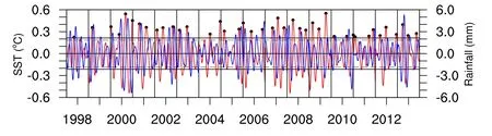
Fig.3.Time series of the 30–60-day filtered SST(red curve;units: °C;left-hand y-axis)and rainfall(blue curve;units:mm;right-hand y-axis)averaged over the rectangle(7°–22°N,109°–120°E)in Fig.2a during boreal summer(May–September)from 1998 to 2013.The parallel dashed lines represent one standard deviation(±0.209°C)of the intraseasonal SST anomaly time series.A strong intraseasonal SST event is defined as a cycle in which the maximum positive SST anomaly exceeds one standard deviation.Black dots show the selected strong events,with each dot indicating the date when the maximum positive SST anomaly occurs in the event.
Figure 3 displays the time series of the area-averaged 30–60-day filtered SST anomalies over the rectangular domain.Strong oscillations of intraseasonal SST anomalies are present in most summers,with the amplitude ranging from at least −0.5°C to+0.6°C.Note that such intraseasonal SST oscillations exhibit considerable year-to-year differences.Given that the intraseasonal precipitation–SST relationship can reflect the air–sea interaction to some extent(Roxy and Tanimoto,2012),the time series of the areaaveraged 30–60-day filtered precipitation anomalies is also shown in Fig.3.It is found that the positive SST anomalies generally lead the positive precipitation anomalies by around 10 days(a phase lag of 1/4 period of the 30-60-day oscillation),while the positive SST anomalies lag the negative precipitation anomalies by 10 days(as discussed below).
3.2.Structure and evolution of the 30–60-day SST variability
To examine the spatial pattern and evolution of the 30–60-day SST fluctuation in relation to the atmospheric forcing,phase compositing is applied to strong intraseasonal SST events that are identified using the area-averaged 30–60-day filtered SST time series(Fig.3).Following Roxy and Tanimoto(2012),a strong intraseasonal SST event is defined as a cycle in which the maximum positive SST anomaly exceeds one standard deviation from zero.In each event,the date of the maximum SST occurrence is designated as Day 0,with the days before(after)the Day 0 labeled as negative(positive)days.As such,a strong intraseasonal SST event characterized by a cycle from −20 days(Day−20)to+20 days(Day+20)relative to Day 0 corresponds to the mean period of a 30–60-day oscillation.As a result,there are 41 strong intraseasonal SST events identified from 1998 to 2013.
Figure 4 shows the composite evolutions of the 30–60-day filtered SST and precipitation during a strong intraseasonal SST event,and Fig.5 displays the composite patterns of intraseasonal SST and surface winds.On Day−20(Figs.4a and 5a),statistically significant negative SST anomalies less than−0.2°C are observed in the entire SCS,accompanied by significant anomalous southwesterlies.Note that anomalous southwesterlies flow out from the central-western SCS,inevitably inducing stronger upwelling there,thus resulting in much cooler SST anomalies below −0.3°C,in agreement with Xie et al.(2003).On the other hand,such negative SST anomalies along with divergent southwesterlies certainly inhibit active convection,so there are no significant precipitation anomalies except in the northeastern corner of the SCS.Five days later(Fig.4b),significant negative precipitation anomalies appear over the southern SCS,with anomalous easterlies occurring over the equatorial region and anomalous southwesterlies retreating to the northern coastal area of the SCS(Fig.5b).Because the decreased precipitation favors increasing surface shortwave radiation(Roxy and Tanimoto,2012),the local SST tends to rise.As a consequence,significant positive SST anomalies develop in the southern SCS,while negative SST anomalies disappear in the northern SCS(Fig.4c).The formation of the positive SST anomalies is also related to anomalous northeasterlies between the anomalous cyclone over the equatorial region and the anticyclone over the northern SCS(Fig.5c).Since the anomalous northeasterlies tend to weaken the summertime background southwesterlies,the surface evaporation is reduced.This effect of reduced evaporation also favors SST warming.Note that positive(negative)precipitation anomalies correspond to the anomalous cyclone over the equatorial region(the northern SCS),and such a meridional dipole structure is actually the zonally elongated monsoonal trough–ridge seesaw pattern identified by Mao and Chan(2005).
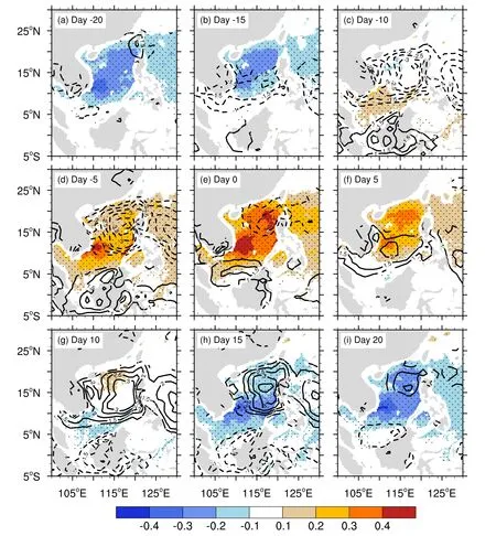
Fig.4.Composite evolution of the 30–60-day filtered SST(shading;units:°C)and precipitation(contours;units:mm;interval:0.5 mm)during a strong intraseasonal SST event at five-day intervals from(a–i)Day −20 to Day 20.Stippling denotes SST anomalies statistically significant at the 99%confidence level.The thick solid(dashed)curves represent positive(negative)precipitation anomalies statistically significant at the 99%confidence level.
Subsequently,both positive and negative precipitation anomalies are enhanced(Fig.4d),as the trough–ridge seesaw circulation pattern migrates northward(Fig.5d).The intensified northeasterlies further reduce the surface evaporation,facilitating the increase in SST.Note that a center with SST anomalies above 0.3°C is forming in the central-western SCS,as was identified by Roxy and Tanimoto(2012),who only used this central-western SCS as the key area to define strong intraseasonal SST events.Meanwhile,the enhanced negative precipitation anomalies over the northern SCS represent locally enhanced descending motion,which leads to increased shortwave radiation and hence a rise in local SST(Fig.4d).During this period from Day−10 to Day−5,there appears to be positive feedback between the increased SST and enhanced dipole circulation:the warmer SST in the southern SCS inevitably induces stronger upstream northeasterlies converging toward the warm region,further reducing surface evaporation and enhancing surface shortwave radiation,so the positive SST anomalies increase further.On the other hand,as suggested by Gill(1980),intensification of the anomalous northeasterlies may be partly attributable to the wind response to equatorial convective heating and atmospheric radiation cooling over the northern SCS corresponding to the trough–ridge seesaw pattern(Figs.4d and 5d).The positive feedback continues so that the positive SST anomalies reach their maximum over the entire SCS on Day 0(Figs.4e and 5e),forming an opposite pattern to that at Day−20(Figs.4a and 5a).In turn,the warmed SCS causes the surrounding air to converge such that on Day 5 anomalous southwesterlies are produced over the southern SCS(Fig.5f)together with positive precipitation anomalies(Fig.4f).The positive precipitation anomalies,representing active convection,tend to reduce the surface shortwave radiation,leading to local SST cooling.In addition,through the thermally forced response(Gill,1980)to active convective heating over the southern SCS,the anomalous southwesterlies are again intensified and migrate further northward.Subsequently,the enhanced southwesterlies in turn increase surface evaporation again,and less shortwave radiation reaches the surface,returning to the minimum state with negative SST anomalies by Day 20(Figs.4i and 5i).

Fig.5.As in Fig.4 but for 30–60-day filtered SST(shading;units:°C)and surface winds(vectors;units:m s−1).Thick vectors indicate that at least one of the zonal and meridional wind anomalies is statistically significant at the 99%confidence level.
The above analyses suggest that the 30–60–day intraseasonal variability of SST in the SCS is characterized by the alternate occurrence of basin-wide positive and negative SST anomalies,with positive(negative)SST anomalies accom-panied by anomalous northeasterlies(southwesterlies).The transformation from positive(negative)to negative(positive)SST anomalies begins in the southern SCS,and then the SST anomalies expand northward to the entire SCS.The transition and expansion of SST anomalies are actually driven by the northward-migrating trough–ridge seesaw circulation pattern from the equator to the northern SCS.Here,the atmosphereto-ocean effect is highlighted in driving strong intraseasonal SST fluctuations.
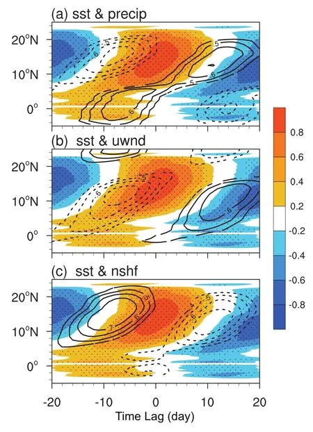
Fig.6.(a)Time-lag–latitude diagram(110°–120°E)of correlation coefficients of the 30–60-day filtered SST(color shading)and precipitation(contours;interval:0.2)anomalies against the area-averaged 30–60-day filtered SST anomaly over the rectangle(7°–22°N,109°–120°E)for the 1998–2013 boreal summers(May–September).The abscissa refers to the time lag(day).Stippling indicates that correlation coefficients between SST anomalies are statistically significant at the 95%confidence level.The zero line is omitted.Thick contours denote the correlation coefficients between SST and precipitation anomalies are statistically significant at the 95%confidence level.(b)As in(a)but for SST and surface zonal wind anomalies.(c)As in(a)but for SST and NSHF anomalies(downward is positive).
To further examine how intraseasonal SST anomalies propagate northward coherently due to atmospheric thermodynamic forcing,Fig.6 shows the time-lagged correlations of the area-averaged 30–60-day filtered SST with intraseasonal SST,precipitation,surface zonal wind,and NSHF anomalies.Looking first at the correlation distributions of intraseasonal SST anomalies at different latitudes with the area-averaged SST reference time series,significant positive and negative correlations are observed to occur alternately at different time lags,with the maximum positive(negative)correlations between 10°N and 20°N around Day 0(Day −20 and Day 20)(Figs.6a–c).The originating positive(negative)correlations can be traced back to the equatorial region around Day−10(Day 10),indicating that the intraseasonal SST signals propagate northward coherently from the equatorial region to the northern SCS.The significant precipitation signals correlated with anomalous SST also exhibit coherent northward migration from the southern SCS,with maximum negative(positive)correlation occurring when SST lags(leads)precipitation by 10 days(Fig.6a).Note that the SST–precipitation correlations show a distinct out-of-phase variation between the equatorial region and the northern SCS,reflecting the trough–ridge seesaw pattern(Figs.4 and 5).The SST–zonal wind correlations indicate that anomalous easterlies(westerlies)originate from the equatorial region and then propagate northward as far as around 18°N(Fig.6b),with maximum negative(positive)correlation appearing when SST lags(leads)zonal wind by 7(13)days.The SST–NSHF correlations demonstrate that anomalous NSHF,as a dominant contributor to the formation of SST anomalies,propagates northward in a similar manner to anomalous precipitation(Fig.6c).This is because positive(negative)NSHF anomalies mostly result from negative(positive)precipitation anomalies.
Given that the NSHF is the most important thermodynamic factor directly affecting the SST tendency,the correlations of area-averaged SST with each NSHF component are again calculated(Fig.7).The anomalous downward surface shortwave radiation flux is the largest component of the NSHF anomalies,and depends on the precipitation anomalies,so anomalous shortwave radiation flux exhibits similar northward propagation to anomalous NSHF(Fig.7a).However,the surface latent heat flux anomalies do not show evident northward propagation(Fig.7b).Although the magnitudes of longwave radiation flux and sensible heat flux anomalies are usually less than the downward shortwave radiation,their correlations with the area-averaged SST anomaly demonstrate that the anomalous signals of these two components also propagate northward considerably from the equator to the northern SCS(Figs.7c and 7d).Note that the time lags are also different from those of downward shortwave radiation anomalies.
4.Heat budget diagnosis for the 30–60-day SST variability
4.1.Relative contribution to intraseasonal SST tendency

Fig.7.As in Fig.6 but for(a)SST and surface shortwave radiation flux anomalies,(b)SST and surface latent heat flux anomalies,(c)SST and longwave radiation flux anomalies,and(d)SST and sensible heat flux anomalies.Downward is positive for each flux component.
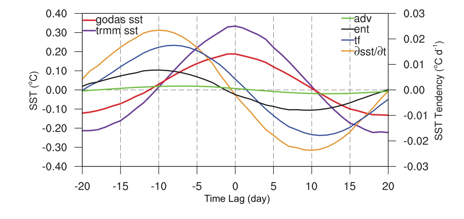
Fig.8.(a)Time series of composite area-averaged 30–60-day filtered TRMM-based SST(purple curve;units:°C;left-hand y-axis)and GODAS mixed-layer temperature as a proxy of SST(red curve;units: °C;left-hand y-axis)and total SST tendency(yellow curve;units: °C d−1;right-hand y-axis)over the rectangle(7°–22°N,109°–120°E)during a strong intraseasonal SST event from Day−20 to Day 20.Also shown are the SST tendency components due to MNHF-related thermal forcing(blue curve;units:°C d−1),vertical entrainment(black curve;units:°C d−1),and horizontal temperature advection(green curve;units:°C d−1).
As suggested by Duvel et al.(2004)and Huang et al.(2010),the SST variations are closely related to perturbations of the average mixed-layer temperature.Thus,the mixedlayer temperature equation,Eq.(1),is used to diagnose the intraseasonal SST variability in the SCS based on GODAS oceanic reanalysis data.Figure 8 illustrates the composite evolutions of the area-averaged 30–60-day filtered SST anomaly and its local tendency,together with the intraseasonal SST tendency from each of the first three terms on the right-hand side of Eq.(1).The total intraseasonal SST tendency(indicated by ∂SST/∂tin Fig.8)takes the form of a regular sinusoid within a 30–60-daycycle,while the evolution of the SST anomaly,obtained by integrating the tendency,follows a cosine curve ranging from −0.15°C to 0.20°C.Note that the varying amplitude of the intraseasonal SST represented by the GODAS mixed-layer temperature is evidently less than that of the intraseasonal TRMM-based SST,and this is because the former represents the averaged temperature of the mixed layer below the sea surface.As suggested by Duvel and Vialard(2007),another reason is that most oceanic reanalysis data tend to underestimate the intraseasonal SST variability.
In Fig.8,the intraseasonal SST tendency components caused by the MNHF-related thermal forcing,horizontal advection,and vertical entrainment exhibit distinct differences in magnitude.The MNHF-generated local change rate has the largest amplitude,indicating that the MNHF-related forcing is indeed the major contributor to the total intraseasonal SST tendency.The second largest contribution comes from the vertical entrainment,with amplitude comparable to that from the MNHF-related forcing.The amplitude of the SST tendency component caused by the horizontal temperature advection is close to zero,suggesting its minor contribution to intraseasonal SST fluctuations.
Note also that the positive SST tendency reaches its maximum around Day−10(Fig.8).Figure 9 presents the spatial distributions of mixed-layer heat budgets associated with the SST tendency from Day−10 to Day 10,in order to demonstrate in detail the spatial coherence of the evolution of SST tendencies and the importance of the MNHF-related forcing and vertical entrainment in strong intraseasonal SST variability.
On Day−10,significantly positive total SST tendencies are present over almost the entire SCS,with maximum rates exceeding 0.04°C d−1in the central-western SCS(Fig.9a).The pattern of the significant SST tendency components caused by MNHF-related forcing(Fig.9b)is similar to that due to the vertical entrainment(Fig.9d),except that the maxima of the latter are slightly less than those of the former.The SST tendency due to horizontal temperature advection(Fig.9c)is less statistically significant.Note from Fig.5c that on Day−10 an anomalous anticyclone dominates the SCS,which certainly enhances the downward surface solar shortwave radiation that heats the upper ocean(Fig.9b).Meanwhile,such anticyclonic wind-stress curl inevitably leads to strong oceanic downwelling(Fig.9d).The strong anomalous northeasterlies on the southern side of the anticyclone(Fig.5c)also intensify oceanic downwelling,especially in the western SCS(Fig.9d).
By Day−5,the total SST tendencies and their components decrease and retreat northward(Figs.9e–h)as the anomalous anticyclone migrates northward(Fig.5d).When anomalous northeasterlies prevail over the entire SCS on Day 0(Fig.5e),significantly negative SST tendencies occur in the southern SCS(Figs.9i–l),especially that associated with oceanic upwelling driven by cyclonic wind-stress curl(Fig.9l).As the anomalous cyclone gradually dominates the SCS from Day 5 to Day 10(Figs.5f and g),the maximum negative SST tendencies occupy the entire SCS on Day 10(Figs.9q–t),forming similar patterns but with opposite sign to Day−10(Figs.9a–d).
To further distinguish the relative importance of individual sub-terms associated with MNHF-related forcing,horizontal advection,and vertical entrainment,the area-averaged SST tendency due to each sub-term on Day−10 is shown in Fig.10.The tendency due to mixed-layer net shortwave radiation forcing is 0.013°C d−1,which accounts for 57.8%of the total SST tendency in the transition phases of the intraseasonal SST event.Next is the latent heat flux forcing,with a tendency of around 0.004°C d−1.These results again highlight the importance of the thermal forcing associated with the solar shortwave radiation and latent heat fluxes relative to the other thermal forcing terms,as in Fig.9b.The areaaveraged SST tendency component caused only by the entrainment is 0.009°C d−1on Day −10,reaching as much as 34.5%of the total tendency(Fig.10).For some strong intraseasonal SST events,the entrainment may contribute as much as the MNHF-related forcing(as discussed below).These results substantiate quantitatively the importance of the vertical entrainment in generating strong intraseasonal SST variations in the SCS,as suggested by Wu et al.(2015).
4.2.Case study highlighting the importance of vertical entrainment
Although the composite evolutions in Figs.8 and 9 indicate that the magnitude of the entrainment-induced intraseasonal SST tendency is usually less than that of the MNHF-induced tendency,exceptions may occur in some specific strong intraseasonal SST events because the strong events vary from summer to summer,as shown in Fig.3.We therefore select typical cases in 2011 to further demonstrate the importance of vertical entrainment in the development of strong intraseasonal SST variability.These representative cases are chosen because the SST fluctuations were less dominated by the surface thermal forcing.This is shown by the relatively small amplitude of anomalous precipitation in summer 2011 compared with other summers(Fig.3),as oceanic processes are thought to play a greater role in intraseasonal SST variability when the NSHF contribution to intraseasonal SST fluctuations is not large(Wu et al.,2015).
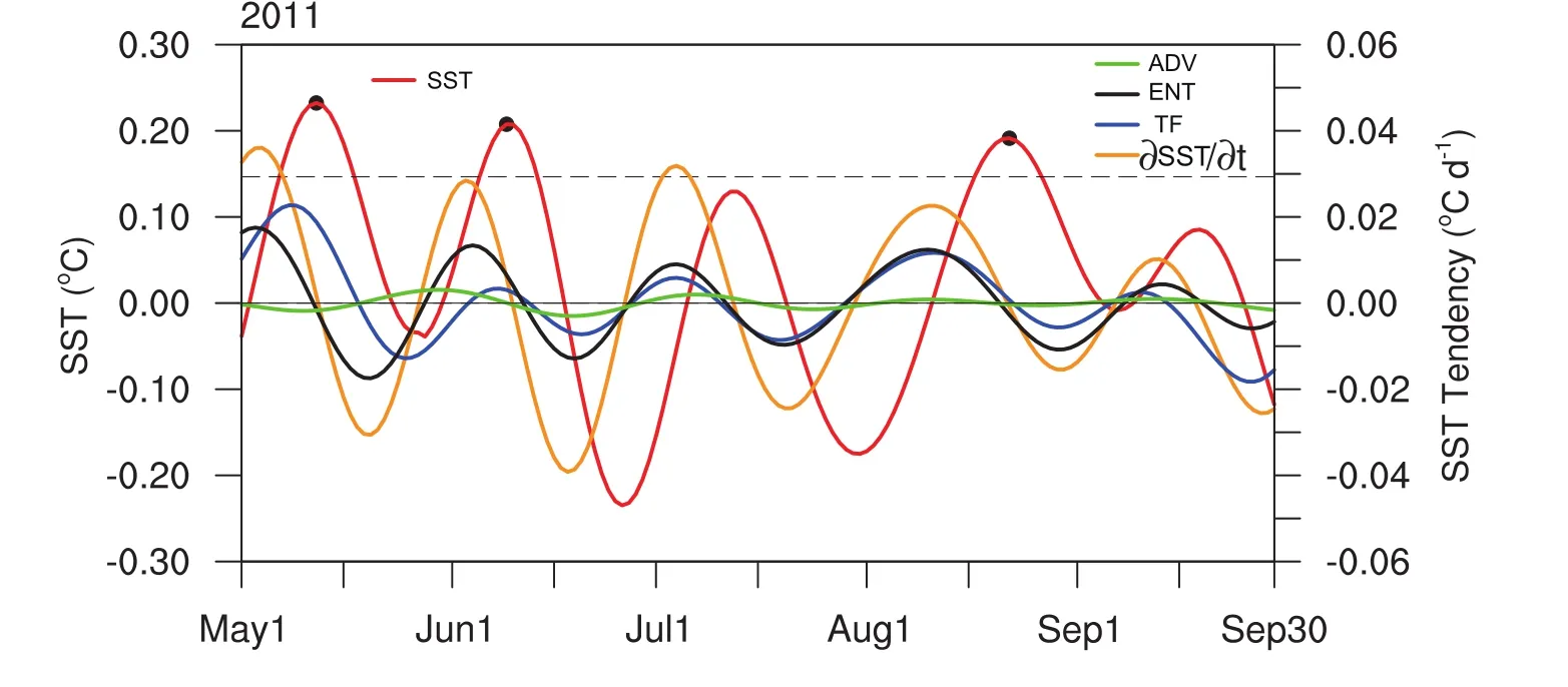
Fig.11.As in Fig.8 but for summer 2011 from 1 May to 30 September.The horizontal dashed line represents the threshold of one standard deviation for the intraseasonal SST(actually,the GODAS mixed-layer temperature)anomaly time series,as calculated over summer 2011.Black dots show the strong intraseasonal SST events,with each dot indicating the date when the maximum positive SST anomaly occurs in the event.
Figure 11 illustrates the time series of the area-averaged 30–60-day filtered SST(actually represented by the mean mixed-layer temperature derived from GODAS data)and its tendency contributions from MNHF-related forcing,horizontal temperature advection and vertical entrainment during the summer of 2011.Note from Fig.11 that such GODAS-based intraseasonal SST exhibited similar fluctuations to the TRMM-based TMI SST in 2011(Fig.3),with five maxima occurring on 11 May,9 June,12 July,22 August,and 19 September.Likewise,the standard deviation is again calculated only for the GODAS-based SST anomaly time series during the summer of 2011.According to the threshold of one standard deviation,three cycles,peaking on 11 May,9 June and 22 August,can be identified as strong intraseasonal SST events(Fig.11).In Fig.11,the entrainmentinduced SST tendency component is at least as large as the MNHF-related forcing component for all three strong intraseasonal SST events.For the third strong SST event from 31 July to 7 September,with a peak on 22 August,the entrainment-induced intraseasonal SST tendency is equal to(even larger than)that caused by MNHF-related forcing for the SST warming(cooling)episode.In addition,the contributions from other factors,such as horizontal temperature advection and other subgrid processes[Rin Eq.(1)]are all near zero.The detailed evolution of the mixed-layer heat budget is shown in Fig.12 as spatial distributions over periods of maximum SST from 12 August to 1 September 2011 within this typical strong case.The positive SST tendency occurs on 12 August in the SCS and is replaced by the maximum negative SST tendency on 1 September after half a period of the 30-60-day SST oscillation.In Fig.12,the entrainment-induced intraseasonal SST tendency is as large in magnitude as that caused by MNHF-related forcing,especially on 12 August and 1 September,which is different from the composite patterns(Fig.9).These results demonstrate that the oceanic dynamics associated with vertical entrainment is sometimes the most important process for generating strong intraseasonal SST variability in the SCS.
5.Summary and discussion
This study extends the work of both Roxy and Tanimoto(2012)and Wu et al.(2015)to characterize the 30–60-day intraseasonal SST variability in the SCS during boreal summer(May–September).Using TRMM-based SST,TropFlux,GODAS oceanic reanalysis,and ERA-Interim atmospheric reanalysis datasets from 1998 to 2013,we quantitatively investigate the atmospheric thermodynamic and oceanic dynamic mechanisms responsible for the formation of such a 30–60-day SST variability via a diagnosis of the upper-ocean heat budgets.
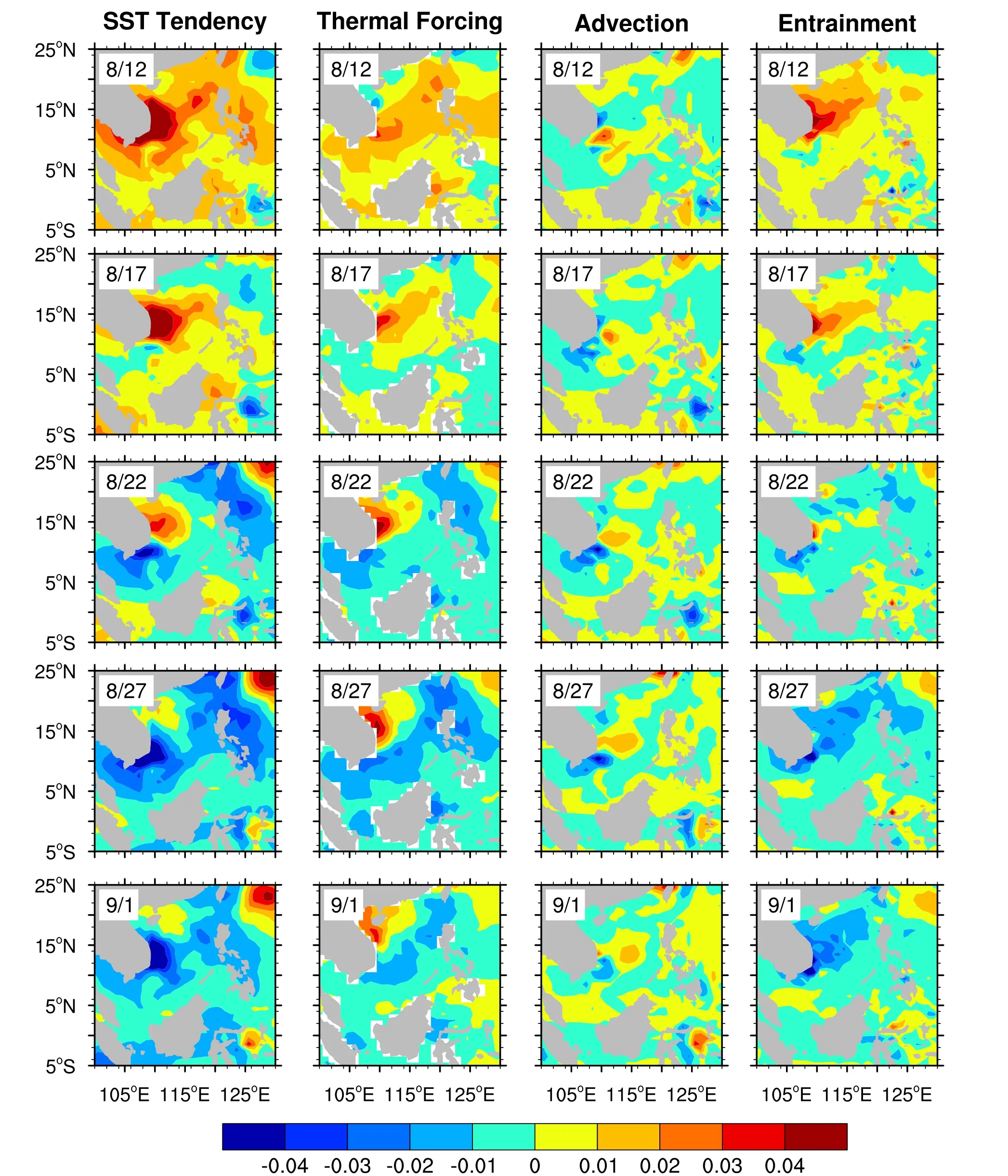
Fig.12.As in Fig.9 but for the period from 12 August to 1 September 2011,within the third strong intraseasonal SST event shown in Fig.11.
Strong intraseasonal SST variability is observed during boreal summer,with the amplitude of the 10–90-day filtered TRMM-based SST exceeding 0.5°C over almost the entire SCS.Power spectrum analysis demonstrates that the 30–60-day component of the intraseasonal SST predominates over the 10–20-day component,with the 30–60-day SST variability explaining more than 60%of the variance of the 10–90-day SST variability for most of the SCS,and even above 70%in the central-western sub-region.Thus,the area-averaged 30–60-day filtered SST over a large domain(7°–22°N,109°–120°E)is used as an index to reflect how the intraseasonal SST overall oscillates over time and to identify the strong intraseasonal SST events.Strong fluctuations of the 30–60-day intraseasonal SST are present in most summers,with considerable interannual differences in amplitude.
Composite analysis of strong intraseasonal SST events is used to examine the spatial pattern and temporal evolution of the 30–60-day SST fluctuation in the SCS in association with atmospheric forcing.The 30–60-day SST variability in the SCS is found to be characterized by the alternate occurrence of basin-wide positive and negative SST anomalies,with positive(negative)SST anomalies accompanied by anomalous northeasterlies(southwesterlies).Furthermore,such anomalous winds are related to a zonally elongated trough–ridge seesaw pattern with an anomalous cyclone coupled with an anomalous anticyclone in the meridional direction.The change from positive(negative)to negative(positive)SST anomalies begins in the southern SCS, and then the SST anomalies expand northward to the entire SCS.The transition and expansion of SST anomalies are actually driven by the trough–ridge seesaw circulation pattern that migrates northward from the equator to the northern SCS,indicating an atmosphere-to-ocean effect in forming strong intraseasonal SST fluctuations.It should be emphasized that the development of the maximum 30–60-day intraseasonal variability in the central-western SCS is also associated with the enhancement of the local oceanic upwelling(downwelling)effect due to the anomalous southwesterlies(northeasterlies)flowing out from(converging on)the central-western SCS,leading to much cooler(warmer)SST anomalies.With a mixed-layer framework,on the other hand,the oceanic upwelling/downwelling again changes the intraseasonal SST anomalies through altering the mixed-layer depth.
The lead–lag correlations of area-averaged 30–60-day filtered SST with intraseasonal surface zonal wind,precipitation,and NSHF con firm that the intraseasonal SST signals propagate northward coherently from the equatorial region to the northern SCS,with maximum negative(positive)correlation appearing when SST lags(leads)zonal wind by 7(13)days,and maximum negative(positive)correlation occurring when SST lags(leads)precipitation by 10 days.As the NSHF is the most important thermodynamic factor driving the local SST tendency,the SST–NSHF correlations show a similar northward propagation to anomalous precipitation,because positive(negative)NSHF anomalies mostly result from negative(positive)precipitation anomalies.However,the surface latent heat flux anomalies do not show evident northward propagation.
Quantitative diagnoses of the mixed-layer heat budgets for the intraseasonal SST variability using GODAS oceanic reanalysis data show that,within a strong 30–60-day cycle,the MNHF-induced SST tendency component exhibits the largest amplitude and its magnitude is comparable to the total intraseasonal SST tendency,with the contribution of anomalous downward net shortwave radiation flux to the total increasing(cooling)rate in the transition phases of the intraseasonal SST event reaching around 60%,indicating that the atmospheric thermal forcing is indeed a dominant factor in driving the strong intraseasonal SST variability.Vertical entrainment is the second most dominant factor,contributing more than 30%to the total intraseasonal SST tendency of the composite situation.However,the entrainment-induced intraseasonal SST tendency may not always be less than that due to MNHF-related forcing.Sometimes,as in the typical strong case from 31 July to 7 September 2011,it is equal to or even larger than the MNHF-induced SST tendency in the transition episodes of the intraseasonal SST event,suggesting that the oceanic dynamics associated with vertical entrainment sometimes plays the leading role in generating strong intraseasonal SST variability in the SCS.
Given the close relationship between the strong local 30–60-day SST variability and the northward-propagating trough–ridge flow pattern,the relative importance of the vertical entrainment could be tested with a suitable SCS regional model in the future,in which the SCS domain is alternately forced with and without the strong influence of intraseasonal atmospheric dynamical fields propagating northward.In addition,10–20-day SST variability may be significant in some summers,and the related physical mechanisms also need to be examined.
Acknowledgements.The TRMM-based TMI SST data are produced by Remote Sensing Systems and sponsored by the NASA Earth Sciences Program,available at http://www.remss.com/missions/tmi.The ERA-Interim data can be downloaded from http://apps.ecmwf.int/datasets/data/interim-full-daily/levtype=sfc/.TheGODASdataareavailableathttp://cfs.ncep.noaa.gov/cfs/godas.The GPCP rainfall data can be downloaded from the databank at http://precip.gsfc.nasa.gov/pub/gpcp-v2/.TropFlux data are produced under a collaboration between Laboratoire d’Oc´eanographie:Exp´erimentation et Approches Num´eriques(LOCEAN),from L’Institut Pierre Simon Laplace(IPSL,Paris,France),and the National Institute of Oceanography/CSIR(NIO,Goa,India),and supported by L’Institut de Recherche pour le D´eveloppement(IRD,France).TropFlux relies on data provided by ERA-Interim and ISCCP.This research was jointly supported by the SOA Program on Global Change and Air–Sea Interactions(Grant No.GASI-IPOVAI-03),the National Basic Research Program of China(Grant No.2014CB953902),the Natural Science Foundation of China(Grant Nos.91537103 and 41375087),and the Priority Research Program of the Chinese Academy of Sciences(Grant Nos.QYZDY-SSWDQC018 and XDA11010402).
Behringer,D.W.,and Y.Xue,2004:Evaluation of the global ocean data assimilation system at NCEP:The Pacific Ocean.Eighth Symposium on Integrated Observing and Assimilation Systems for Atmosphere,Oceans,and Land Surface,Seattle,Washington,Washington State Convention and Trade Center,11–15.
Bellon,G.,A.H.Sobel,and J.Vialard,2008: Oceanatmosphere coupling in the monsoon intraseasonal oscillation:A simple model study.J.Climate,21,5254–5270,https://doi.org/10.1175/2008JCLI2305.1.
Berrisford,P.,P.Kållberg,S.Kobayashi,D.Dee,S.Uppala,A.J.Simmons,P.Poli,and H.Sato,2011:Atmospheric conservation properties in ERA-Interim.Quart.J.Roy.Meteor.Soc.,137,1381–1399,https://doi.org/10.1002/qj.864.
Bretherton,C.S.,M.Widman,V.P.Dymnikov,J.M.Wallace,and I.Blad´e,1999:The effective number of spatial degrees of freedom of a time-varying field.J.Climate,12,1990–2009,https://doi.org/10.1175/1520-0442(1999)012<1990:TENOSD>2.0.CO;2.
Chen,T.-C.,and J.-M.Chen,1995:An observational study of the South China Sea monsoon during the 1979 summer:Onset and life cycle.Mon.Wea.Rev.,123,2295–2318,https://doi.org/10.1175/1520-0493(1995)123<2295:AOSOTS>2.0.CO;2.
Chen,T.-C.,M.-C.Yen,and S.-P.Weng,2000:Interaction between the summer monsoons in East Asia and the South China Sea:Intraseasonal monsoon modes.J.Atmos.Sci.,57,1373–1392,https://doi.org/10.1175/1520-0469(2000)057<1373:IBTSMI>2.0.CO;2.
Chou,C.,and Y.-C.Hsueh,2010:Mechanisms of northward propagating intraseasonal oscillation—A comparison between the Indian Ocean and the western North Pacific.J.Climate,23,6624–6640,https://doi.org/10.1175/2010 JCLI3596.1.
Ding,Y.H.,1994:Monsoons over China.Kluwer Academic Publishers,Dordrecht,Boston,London,419 pp.
Ding,Y.H.,and J.C.L.Chan,2005:The East Asian summer monsoon:An overview.Meteor.Atmos.Phys.,89,117–142,https://doi.org/10.1007/s00703-005-0125-z.
Du,Y.,T.D.Qu,G.Meyers,Y.Masumoto,and H.Sasaki,2005:Seasonal heat budget in the mixed layer of the southeastern tropical Indian Ocean in a high-resolution ocean general circulation model.J.Geophys.Res.,110,C04012,https://doi.org/10.1029/2004JC002845.
Duchon,C.E.,1979:Lanczos filtering in one and two dimensions.J.Appl.Meteor.,18,1016–1022,https://doi.org/10.1175/1520-0450(1979)018<1016:LFIOAT>2.0.CO;2.
Duvel,J.P.,and J.Vialard,2007:Indo-Pacific sea surface temperature perturbations associated with intraseasonal oscillations of tropical convection.J.Climate,20,3056–3082,https://doi.org/10.1175/JCLI4144.1.
Duvel,J.P.,R.Roca,and J.Vialard,2004: Ocean mixed layer temperature variations induced by intraseasonal convective perturbations over the Indian Ocean.J.Atmos.Sci.,61,1004–1023,https://doi.org/10.1175/1520-0469(2004)061<1004:OMLTVI>2.0.CO;2.
Fu,X.H.,B.Wang,T.Li,and J.P.McCreary,2003:Coupling between northward-propagating,intraseasonal oscillations and sea surface temperature in the Indian Ocean.J.Atmos.Sci.,60,1733–1753,https://doi.org/10.1175/1520-0469(2003)060<1733:CBNIOA>2.0.CO;2.
Gill,A.E.,1980:Some simple solutions for heat-induced tropical circulation.Quart.J.Roy.Meteor.Soc.,106,447–462,https://doi.org/10.1002/qj.49710644905.
Gilman,D.L.,F.J.Fuglister,and J.M.Mitchell Jr.,1963:On the power spectrum of “red noise”.J.Atmos.Sci.,20,182–184,https://doi.org/10.1175/1520-0469(1963)020<0182:OTPSON>2.0.CO;2.
Harrison,D.E.,and A.Vecchi,2001:January 1999 Indian Ocean cooling event.Geophys.Res.Lett.,28,3717–3720,https://doi.org/10.1029/2001GL013506.
Huang,B.Y.,Y.Xue,D.X.Zhang,A.Kumar,and M.J.McPhaden,2010:The NCEP GODAS ocean analysis of the tropical Pacific mixed layer heat budget on seasonal to interannual time scales.J.Climate,23,4901–4925,https://doi.org/10.1175/2010JCLI3373.1.
Huffman,G.J.,R.F.Adler,M.M.Morrissey,D.T.Bolvin,S.Curtis,R.Joyce,B.McGavock,and J.Susskind,2001:Global precipitation at one-degree daily resolution from multisatellite observations.Journal of Hydrometeorology,2,36–50,https://doi.org/10.1175/1525-7541(2001)002<0036:GPAODD>2.0.CO;2.
Isoguchi,O.,and H.Kawamura,2006: MJO-related summer cooling and phytoplankton blooms in the South China Sea in recent years.Geophys.Res.Lett.,33(16):L16615,https://doi.org/10.1029/2006gl027046.
Kikuchi,K.,B.Wang,and Y.Kajikawa,2012:Bimodal representation of the tropical intraseasonal oscillation.Climate Dyn.,38,1989–2000,https://doi.org/10.1007/s00382-011-1159-1.
Lau,K.-M.,G.J.Yang,and S.H.Shen,1988:Seasonal and intraseasonal climatology of summer monsoon rainfall over East Asia.Mon.Wea.Rev.,116,18–37,https://doi.org/10.1175/1520-0493(1988)116<0018:SAICOS>2.0.CO;2.
Lau,K.-M.,and S.Yang,1997:Climatology and interannual variability of the Southeast Asian summer monsoon.Adv.Atmos.Sci.,14,141–162,https://doi.org/10.1007/s00376-997-0016-y.
Li,R.C.Y.,and W.Zhou,2015:Multiscale control of summertime persistent heavy precipitation events over South China in association with synoptic,intraseasonal,and low-frequency background.Climate Dyn.,45,1043–1057,https://doi.org/10.1007/s00382-014-2347-6.
Lu,R.Y.,H.L.Dong,Q.Su,and H.Ding,2014:The 30-60-day intraseasonal oscillations over the subtropical western North Pacific during the summer of 1998.Adv.Atmos.Sci.,31,1–7,https://doi.org/10.1007/s00376-013-3019-x.
Mao,J.Y.,and J.C.L.Chan,2005:Intraseasonal variability of the South China Sea summer monsoon.J.Climate,18,2388–2402,https://doi.org/10.1175/JCLI3395.1.
Mao,J.Y.,J.C.L.Chan,and G.X.Wu,2004:Relationship between the onset of the South China Sea summer monsoon and the structure of the Asian subtropical anticyclone.J.Meteor.Soc.Japan,82,845–859,https://doi.org/10.2151/jmsj.2004.845.
Paulson,C.A.,and J.J.Simpson,1977:Irradiance measurements in the upper ocean.J.Phys.Oceanogr.,7,952–956,https://doi.org/10.1175/1520-0485(1977)007<0952:IMITUO>2.0.CO;2.
Praveen Kumar,B.,J.Vialard,M.Lengaigne,V.S.N.Murty,and M.J.McPhaden,2012:TropFlux:Air-sea fluxes for the global tropical oceans-description and evaluation.Climate Dyn.,38,1521–1543,https://doi.org/10.1007/s00382-011-1115-0.
Praveen Kumar,B.,J.Vialard,M.Lengaigne,V.S.N.Murty,M.J.McPhaden,M.F.Cronin,F.Pinsard,and K.Gopala Reddy,2013:TropFlux wind stresses over the tropical oceans:Evaluation and comparison with other products.Climate Dyn.,40,2049–2071,https://doi.org/10.1007/s00382-012-1455-4.
Qu,T.D.,2003:Mixed layer heat balance in the western North Pacific.J.Geophys.Res.,108(C7),3242,https://doi.org/10.1029/2002JC001536.
Reynolds,R.W.,and T.M.Smith,1994:Improved global sea surface temperature analyses using optimum interpolation.J.Climate,7,929–948,https://doi.org/10.1175/1520-0442(1994)007<0929:IGSSTA>2.0.CO;2.
Roxy,M.,and Y.Tanimoto,2012:Influence of sea surface temperature on the intraseasonal variability of the South China Sea summer monsoon.Climate Dyn.,39,1209–1218,https://doi.org/10.1007/s00382-011-1118-x.
Roxy,M.,Y.Tanimoto,B.Preethi,P.Terray,and R.Krishnan,2013:Intraseasonal SST-precipitation relationship and its spatial variability over the tropical summer monsoon region.Climate Dyn.,41,45–61,https://doi.org/10.1007/s00382-012-1547-1.
Wang,B.,F.Huang,Z.W.Wu,J.Yang,X.H.Fu,and K.Kikuchi,2009:Multi-scale climate variability of the South China Sea monsoon:A review.Dyn.Atmos.Oceans,47,15–37,https://doi.org/10.1016/j.dynatmoce.2008.09.004.
Wang,L.,T.Li,and T.J.Zhou,2012:Intraseasonal SST variability and air-sea interaction over the Kuroshio extension region during boreal summer.J.Climate,25,1619–1634,https://doi.org/10.1175/JCLI-D-11-00109.1.
Webster,P.J.,V.O.Magaña,T.N.Palmer,J.Shukla,R.A.Tomas,M.Yanai,and T.Yasunari,1998:Monsoons:Processes,predictability,and the prospects for prediction.J.Geophys.Res.,103(C7),14 451–14 510,https://doi.org/10.1029/97JC02719.
Wentz,F.J.,C.Gentemann,D.Smith,and D.Chelton,2000:Satellite measurements of sea surface temperature through clouds.Science,288,847–850,https://doi.org/10.1126/science.288.5467.847.
Woolnough,S.J.,J.M.Slingo,and B.J.Hoskins,2000:The relationship between convection and sea surface temperature on intraseasonal timescales.J.Climate,13,2086–2104,https://doi.org/10.1175/1520-0442(2000)013<2086:TRBCAS>2.0.CO;2.
Wu,R.G.,2010:Subseasonal variability during the South China Sea summer monsoon onset.Climate Dyn.,34,629–642,https://doi.org/10.1007/s00382-009-0679-4.
Wu,R.G.,and Z.Chen,2015:Intraseasonal SST variations in the South China Sea during boreal winter and impacts of the East Asian winter monsoon.J.Geophys.Res.,120,5863–5878,https://doi.org/10.1002/2015JD023368.
Wu,R.G.,B.P.Kirtman,and K.Pegion,2008:Local rainfall-SST relationship on subseasonal time scales in satellite observations and CFS.Geophys.Res.Lett.,35,L22706,https://doi.org/10.1029/2008GL035883.
Wu,R.G.,X.Cao,and S.F.Chen,2015:Covariations of SST and surface heat flux on 10-20 day and 30-60 day time scales over the South China Sea and western North Pacific.J.Geophys.Res.,120,12 486–12 499,https://doi.org/10.1002/2015JD024199.
Xie,S.-P.,Q.Xie,D.X.Wang,and W.T.Liu,2003:Summer upwelling in the South China Sea and its role in regional climate variations.J.Geophys.Res.,108(C8),3261,https://doi.org/10.1029/2003JC001867.
Zhou,W.,J.C.-L.Chan,and C.Y.Li,2005:South China Sea summer monsoon onset in relation to the off-equatorial ITCZ.Adv.Atmos.Sci.,22,665–676,https://doi.org/10.1007/BF02918710.
杂志排行

Advances in Atmospheric Sciences的其它文章
- Analysis of the Characteristics of Inertia-Gravity Waves during an Orographic Precipitation Event
- Geometric Characteristics of Tropical Cyclone Eyes before Landfall in South China Based on Ground-Based Radar Observations
- Characteristics and Preliminary Causes of Tropical Cyclone Extreme Rainfall Events over Hainan Island
- Numerical Study of the Influences of a Monsoon Gyre on Intensity Changes of Typhoon Chan-Hom(2015)
- Organizational Modes of Severe Wind-producing Convective Systems over North China
- Vortex Rossby Waves in Asymmetric Basic Flow of Typhoons