Regional moment-independent sensitivity analysis with its applications in engineering

Changcong ZHOU,Chenghu TANG,Fuchao LIU,Wenxuan WANG,Zhufeng YUE

School of Mechanics,Civil Engineering and Architecture,Northwestern Polytechnical University,Xi’an,710129,China

Regional moment-independent sensitivity analysis with its applications in engineering

Changcong ZHOU*,Chenghu TANG,Fuchao LIU,Wenxuan WANG,Zhufeng YUE

School of Mechanics,Civil Engineering and Architecture,Northwestern Polytechnical University,Xi’an,710129,China

Available online 8 May 2017

*Corresponding author.

E-mail address:changcongzhou@nwpu.edu.cn(C.ZHOU).

Peer review under responsibility of Editorial Committee of CJA.

Production and hosting by Elsevier

http://dx.doi.org/10.1016/j.cja.2017.04.006

1000-9361©2017 Chinese Society of Aeronautics and Astronautics.Production and hosting by Elsevier Ltd.

This is an open access article under the CC BY-NC-ND license(http://creativecommons.org/licenses/by-nc-nd/4.0/).

Traditional Global Sensitivity Analysis(GSA)focuses on ranking inputs according to their contributions to the output uncertainty.However,information about how the specific regions inside an input affect the output is beyond the traditional GSA techniques.To fully address this issue,in this work,two regional moment-independent importance measures,Regional Importance Measure based on Probability Density Function(RIMPDF)and Regional Importance Measure based on Cumulative Distribution Function(RIMCDF),are introduced to find out the contributions of specific regions of an input to the whole output distribution.The two regional importance measures prove to be reasonable supplements of the traditional GSA techniques.The ideas of RIMPDF and RIMCDF are applied in two engineering examples to demonstrate that the regional moment-independent importance analysis can add more information concerning the contributions of model inputs.

©2017 Chinese Society of Aeronautics and Astronautics.Production and hosting by Elsevier Ltd.This is an open access article under the CC BY-NC-ND license(http://creativecommons.org/licenses/by-nc-nd/4.0/).

Cumulative distribution

function;

Moment-independent;

Probability density function;

Regional importance

measure;

Sensitivity analysis;

Uncertainty

1.Introduction

Sensitivity Analysis(SA)is to study ‘how uncertainty in the output of a model(numerical or otherwise)can be apportioned to different sources of uncertainty in the model input factors”.1Generally,SA can be classified into two main categories1–3:Local Sensitivity Analysis(LSA),which is often carried out in the form of derivative of the model output with respect to the input parameters,and Global Sensitivity Analysis(GSA),which focuses on the output uncertainty over the entire range of the inputs.The limitation of LSA,as a derivative-based approach,lies in that derivatives are only informative at the base points where they are calculated and cannot provide an exploration of the rest of the input space.GSA,on the other hand,explores the whole space of the input factors,and thus is more informative and robust than estimating derivatives at a single point of the input space.Obviously,GSA has a greater potential for engineering applications.

Global sensitivity indices are also known as importance measures,and a rapid development in this field has been witnessed in the last several decades.4The family of importance measures generally includes nonparametric techniques suggested by Saltelli and Marivoet5and Iman et al.,6variance-based methods suggested by Sobol7and further developed by Rabitz and Alis,8Saltelli et al.,9and Frey and Patil,10and moment-independent approaches proposed by Park and Ahn,11Chun et al.,12Borgonovo,13,14Liu and Homma,15and Castaings et al.16It has been found that nonparametric techniques are insufficient to capture the influences of inputs on the output variability for nonlinear models and also when interactions among inputs emerge.10As Saltelli underlined,1an importance measure should satisfy the requirement of being ‘global,quantitative,and model free”,and he advocated that the variance-based importance measure was a preferred way of measuring uncertainty importance.However,the use of variance as an uncertainty measure relies on the assumption that ‘this moment is sufficient to describe output variability”.13Borgonovo13showed that relying on the sole variance as an indicator of uncertainty would sometimes lead a decision maker to noninformative conclusions,since the inputs that influence the variance the most are not necessarily the ones that influence the output uncertainty distribution the most.Borgonovo extended Saltelli’s three requirements by adding ‘moment independent”,13,14and proposed a new importance measure which looks at the influence of the input uncertainty on the entire output distribution without reference to a specific moment of the output.In a similar manner,Liu and Homma15proposed another moment-independent importance measure,which describes the contribution of the input uncertainty on the Cumulative Distribution Function(CDF)of the model output,while Borgonovo’s importance measure studies the contribution on the Probability Density Function(PDF)of the model output.

However,traditional GSA techniques only provide information showing the relative importance of input variables,with no knowledge of which part of a variable is important such as the left or right tail,center region,near center,etc.Such information will be useful for decision makers to identify the important areas inside an input variable,and take corresponding measures.For this purpose,Millwater et al.17proposed a localized probabilistic sensitivity method to determine the random variable regional importance;however,this method is based on derivatives and suffers the same constraints as those of LSA.In 1993,Sinclair18introduced the idea of Contribution to Sample Mean(CSM)plot which was further developed by Bolado-Lavin et al.19As an extension of CSM,Tarantola et al.20proposed the Contribution to Sample Variance(CSV)plot.The principle behind CSM and CSV is to use a given random sample of input variables,which is generally used for uncertainty analysis,to measure the effects of specific regions of an input variable on the mean and variance of the output.However,the information provided by CSM and CSV will become limited when the mean and variance are insufficient to describe the output distribution,which is possible in both theoretical and real applications.

In this work,the idea of CSM and CSV is extended to the domain of moment-independent GSA techniques.Based on the importance measures proposed by Borgonovo13and Liu and Homma15respectively,regional moment-independent importance analysis considering the output PDF and CDF is introduced,to find out the contributions of specific regions of an input variable to the whole output distribution.Besides,the regional importance analysis can be performed with the same sample points for computing the traditional momentindependent importance measures,and thus no additional model evaluation is needed.In other words,the regional moment-independent importance analysis can be viewed as a byproduct,offering much more information than that provided by the standard importance analysis.

The remainder of this paper is organized as follows.The CSM and CSV theories are brief l y reviewed in Section 2.Then the regional moment-independent importance analysis and computational strategies are discussed in Section 3.In tion 4,two engineering examples are presented to demonstrate the applicability of the newly proposed concept.Finally,conclusions of this work are highlighted in Section 5.

2.Review of CSM and CSV plots

Suppose that the input-output model is denoted byY=g（X）,whereYis the model output andX= ［X1，X2，...，Xn］T(nis the input dimension)is the set of input variables.The uncertainties of the input variables are represented by probability distributions.The joint probability density function PDF ofXis denoted asfX（x）,and the marginal PDF ofXican be formulated as

Let us recall the definition of CSM for a given input

根据土地利用现状分类二级小类，参考谢高地[4]、陈士银[20]、张天海[16]等人确定的生态系统类型进行合并划分，将苏州市土地分为耕地、园地、林地、牧草地、城乡建设用地、交通用地、水域、未利用地8类用地（图2）。

whereq∈ ［0，1］,E（Y）=of the model output,andis the inverse CDF ofXiat quantileq.The multiple integral in Eq.(2)is taken in the range（-∞，+∞）for all the input variables exceptXi,for which the range is

In a similar manner,CSV forXiis defined as20

whereV（Y）=the variance of the model output,and the other notations have the same meaning as in the definition of CSM.It is important to note that CSV is defined as a contribution to the output variance with respect to a constant meanE（Y）over the full range.

Both CSM and CSV are plotted in the ［0，1］2space,withqas a point onx-axis representing a fraction of the distribution range ofXi,and CSMXi（q）or CSVXi（q）as a fraction of the output mean or variance corresponding to the values ofXismaller than or equal to itsqquantile.

CSM and CSV are meaningful to estimate the contributions of specific ranges of an input variable to the mean and variance of the output.ConsideringXiand a specific range ofq,say［0，0.1］for example,if the CSM or CSV plot is close to the diagonal,it indicates that the contribution to the output mean or variance is almost equal throughout this range ofXi.In addition,the contribution ofXiin the range to the output mean or variance is lower than the average if the CSM and CSV plots are convex downwards;otherwise,the contribution is higher than the average if the plots are convex upwards.Furthermore,considering another range ［q1，q2］ofXi,the values of CSMXi（q2）-CSMXi（q1）or CSVXi（q2）-CSVXi（q1）can measure the contribution of this range to the output mean or variance.Clearly,CSM and CSV provide much more information than solely performing the standard GSA techniques,along with the convenience that the plots can be depicted without additional model evaluations.Readers are referred to Refs.18–20for more detailed proofs and interpretations of CSM and CSV.

3.Regional moment-independent importance analysis

3.1.Two moment-independent importance measures

Instead of evaluating the output uncertainty only by the mean or variance,the moment-independent importance analysis estimates the contributions of input variables on the whole output distribution.In this work,we extend the idea of regional sensitivity analysis to two moment-independent importance measures considering the PDF and CDF of the output.The unconditional PDF and CDF of the model outputYare denoted asfY（y）andFY（y）,respectively.The conditional PDF and CDF ofYare denoted asfY｜Xi（y）andFY｜Xi（y）,which can be obtained by fixing the input of interestXiat its realizationgenerated by its distribution.The conditional and unconditional distribution functions of the output are depicted in Fig.1.

Borgonovo13proposed his importance measure by considering the contributions of inputs to the PDF of the model output.The shift betweenfY（y）andfY｜Xi（y）is measured by the areas（Xi）closed by the two PDFs,which is given as

The expected shift can be obtained by varying the value ofXiover its distribution range,i.e.,

Then Borgonovo’s importance measure is defined as

In a similar manner,Liu and Homma15proposed a new moment-independent importance measure considering the CDF of the model output.The deviation ofFY｜Xi（y）fromFY（y）is measured by using the areaA（Xi）closed by the two CDFs,and can be calculated as

The expected deviation ofFY｜Xi（y）fromFY（y）can be obtained as

EXi［A（Xi）］can be utilized to illustrate the influence of the inputXion the output distribution.Liu and Homma15defined this measure as the CDF-based sensitivity indicator and denoted it as.Furthermore,for a general model of which the unconditional expectation of the outputE（Y）is not equal to 0,can be normalized as

Both δiandevaluate the influence of the entire distribution of the inputXion that of the model outputY,except that the former focuses on the PDF of the output while the latter focuses on the CDF.For both measures,the effect ofXion the output uncertainty is estimated by varying all the other inputs over their variation ranges.The two momentindependent importance measures represent the expected shift in a decision maker’s view on the output uncertainty provoked byXi.The inputs with larger values of δiorwill be associated with a higher importance,indicating that these inputs should be paid more attention to if we want to control the model performance.In fact,the two measures work regardless of whether the model is linear or nonlinear,additive or nonadditive,and can be easily extended to a group of inputs,for which more detailed information can be found in the works of Borgonovo13,14and Liu and Homma.15

3.2.Regional importance analysis based on δiand

The two measures,δiand,add new insights into the GSA.However,just like the other GSA techniques,both measures can only estimate the contribution of the entire input distribution to the output uncertainty.In this respect,we consider to extend the idea of CSM and CSV to δiand,and propose a new concept of regional moment-independent importance analysis.

Just like the way of defining CSM and CSV,instead of integratings（Xi）at （-∞，+∞）in Eq.(5),we cut the integration range down to （-∞，（q）］for investigating the contribution ofXiwithin this range to the output PDF.We now put forward the Regional Importance Measure based on PDF(RIMPDF),and present its formulation as

RIMPDFXi（q）can be plotted in the ［0，1］2space.Compared to δiwhich can rank the inputs according to their contributions,RIMPDFXi（q）is able to further investigate the effects that specific areas of an input have on the output PDF.In fact,a similar idea of considering the regional effects of the inputs on δiwas also discussed by Wei et al.21;however,in this work,it is discussed in a different and more comprehensive way.

Similarly,the Regional Importance Measure based on CDF(RIMCDF),can be established as

RIMCDFXi（q）is also plotted in the ［0，1］2space,and it investigates the contributions of specific areas of an input variable to the output CDF.

Obviously,RIMPDFXi（q） andRIMCDFXi（q） canbe viewed as regional versions of the two moment-independent measures δiand.However,it is very meaningful to perform such extensions,as RIMPDFXi（q）and RIMCDFXi（q）can act as good supplements to δiand,and enrich the available information by moment-independent importance analysis.Besides,they can be easily estimated by using the same samples for evaluating δiand,and thus no additional model evaluation is needed,which will be discussed later in this work.

3.3.Interpretations of RIMPDFXi（q）and RIMCDFXi（q）

The newly proposed regional measures,RIMPDFXi（q）and RIMCDFXi（q）,can be interpreted similarly as CSM and CSV,except that the former two consider the whole output distribution while the latter only consider the first two moments of the output.If the plot of RIMPDFXi（q）or RIMCDFXi（q）is close to the diagonal,it means that the contribution of the input variable to the output PDF or CDF is nearly unvarying in its current range.If the plot is convex upwards,it means that in this range,the input variable contributes more than the average to the output PDF or CDF;otherwise,the contribution is lower than the average if the plot exhibits an opposite trend.

Furthermore,some interesting properties of these two regional moment-independent importance measures are noticed and listed as follows.

Important information can be provided by Property III:given the quantilesq1andq2,reduction of the two momentindependent importance measures by reducing the range ofXifrom （-∞，+∞）to ［xi，1，xi，2］can be estimated by Eqs.(12)and(13).Sinceq1andq2can be any value from the interval［0，1］as long as satisfyingq1＜q2,a 3D plot can be created indicating the region where the reduction of the input contribution to the whole output distribution can be most effectively achieved.Obviously,such information will be missed if only performing the traditional importance analysis reviewed in Section 3.1.

Properties I and II can be easily derived by the definitions of regional importance measures,and here we only give the proof of Property III.

Proof.Let us consider the input variableXiwith its PDFfXi（xi）over （-∞，+∞）.Now the range ofXiis reduced to［xi，1，xi，2］(corresponding to the quantile interval ［q1，q2］),and according to the principles of truncated distribution,the PDF ofXiafter the reduction can be established as20

Then Borgonovo’s and Liu’s importance measures ofXiafter the distribution reduction can be computed as

Meanwhile,the following equations hold by Eqs.(10)and(11):

Property III is readily obtained based on Eqs.(19)and(20). □

3.4.Computational strategies

The moment-independent importance measures add necessary tools to the domain of sensitivity analysis for quantifying the contributions of inputs to the model output.Basically,it needs a double-loop sampling procedure to estimate δiandNow we describe the computational method proposed by Borgonovo13to obtain δi.Firstly,the unconditional PDF of the output,fY（y）,is obtained by uncertainty propagation,varying the inputs over their variation ranges.Secondly,one generates a value forXi,namelysampled byfXi（xi）.With this value,the conditional PDF of the output,fY｜Xi（y）,is obtained by propagating uncertainty in the model fixingis computed from the numerical integration of the absolute value of the difference betweenfY｜Xi（y）andfY（y）.Repeat the procedure for a certain number of times,and δican be finally estimated.In fact,the calculation ofcan be implemented in a similar way,only needing to substitute the PDFs in Borgonovo’s method with CDFs.

As we have noted before,the regional importance measures,RIMPDFXi（q）and RIMCDFXi（q）,can be obtained simultaneously when estimating δiand,with the same sample points.Now we describe the generalized steps for estimating regional importance measures.

Step 1.Generate N samplesxt= ［x1t，x2t，...，xnt］（t=1，2，...，N）of the input variables randomly according to the joint distribution,and obtain the corresponding model output values yt.

Step 2.Sort the samples of theith input variablein an ascending order,and compute the corresponding values of s（Xi）and A（Xi）in the way we just described above,denoted as

Step 3.Estimate the regional moment-independent measures for Xias

where ｜qN｜is the largest integer not greater thanqN.

A few comments need to be added here.In the second step,when computing the values ofs（Xi）andA（Xi）withXifixed at one sample point,estimation of PDF and CDF is involved.In this work,a new adaptive Kernel Density Estimator(KDE)proposed by Botev et al.23is adopted to estimate PDF and CDF.According to the steps described above,a total ofnN2times of model evaluations is needed to perform the regional moment-independent importance analysis.Obviously,the computational burden may become unbearable in some applications if the model evaluation is rather time-consuming.Now let us consider if there is any more efficient way to perform such analysis.

Recently,Wei et al.24has developed a sing-loop Monte Carlo method to estimate Borgonovo’s importance measure,δi.This method proves to be rather efficient with acceptable accuracy.Noting thatfY｜Xi（y）=fY，Xi（y，xi）/fXi（xi）,the following transformation is proposed by Wei et al.24:

wherefY，Xi（y，xi）is the joint PDF of the model outputYand the input variableXi.By such a transformation,estimation of δiturns to be a single-loop procedure,which will cut down the computational efforts remarkably.The robustness of this method has been demonstrated by Wei et al.24It can be seen that the final formulation in Eq.(23)can be easily calculated by the Monte Carlo simulation method except that the marginal PDFfY（y）and the joint PDFfY，Xi（y，xi）need to be estimated.

Similarly,we can do a similar transformation toas

AfterfY（y）andfY，Xi（y，xi）are estimated,S（CDF）ican be obtained by numerical integration in Eq.(24).It is admitted that in some cases,the numerical integration may be difficult to converge to produce a precise result.Nevertheless,the transformation in Eq.(24)provides an optional way to estimaten a single-loop procedure.

In fact,the single-loop Monte Carlo method for δiandcan be extended to the regional moment-independent importance analysis.The general procedure is summarized as follows:

Step 1.Generate N samplesxt= ［x1t，x2t，...，xnt］（t=1，2，...，N）of the input variables randomly according to the joint distribution,and obtain the corresponding model output values yt.

Step 2.Estimate fY（y）and fY，Xi（y，xi）using the KDE technique proposed by Botev et al.23Sort the sample of Xiin an ascending order asand then the output values are correspondingly sorted as （y（1），y（2），...，y（N））.Calculate the corresponding values of the PDFs at these sample points:

Step 3.For RIMPDF,it can be estimated as

where ｜qN｜is the largest integer not greater thanqN.

However,for RIMCDF,there needs a numerical integration process afterfY（y）andfY，Xi（y，xi）are estimated.It can be formulated as

whereE（Y）can be estimated using the samples in Step 1.

By the procedure described above,the computational burden of regional moment-independent importance is partly eased by a single-loop simulation process.It should be noted that estimation of RIMCDF may become difficult in some cases as numerical integration is involved,and the double-loop method can be used in such cases.Estimation of distribution-based sensitivity indices have long been a tricky issue,and many methods have been studied to address this issue.25–27Nevertheless,the emphasis of this paper is to introduce a novel idea of regional momentindependent importance analysis,and more comprehensive discussions concerning the computational strategies will be made in the upcoming research work.

4.Applications

In this section,the regional moment-independent importance analysis is tested by two engineering examples.The results will be discussed in a detailed manner,to demonstrate the significance of the newly proposed concepts of RIMPDF and RIMCDF.

4.1.Example 1:A riveting process

In the aircraft industry,sheet metal parts are widely used,and riveting is the most common method to assemble them.28,29Many factors have to be considered during the riveting process,which may directly affect the riveting quality.One main factor is the squeeze force.If the squeeze force is too low,rivets may be too loose to efficiently join different parts,while a too high squeeze force may induce excessive residual stresses which will result in stress concentrations(around holes and rivets)and initial cracks.Both cases are dangerous for aircraft.Therefore,it is quite necessary to determine the squeeze force properly for the sake of flight safety.

The real riveting process is very complex.In this work,we take a headless rivet as an example,and generalize the riveting process into two stages as shown in Fig.2.In Stage 1,the rivet is punched from State A(the initial state of the rivet before impact,without any deformation)to State B(an intermediate state of the rivet when there is no clearance between the rivet and the hole),and then in Stage 2,the rivet is further punched from State B to State C(the final state of the rivet after impact,with rivet heads formed).Throughout the riveting process,we assume that the hole diameter keeps unchanged.

To establish the relationship between the geometric dimensions of a rivet and the squeeze force,the following ideal conditions should be assumed:

(1)The hole is not enlarged in the riveting process.

(2)The change of the rivet volume in the process can be neglected.

(3)After impact,the rivet driven head has a cylindrical shape.

(4)The material of the rivet is isotropic.

The initial volumeV0of the rivet before the impact(in State A)is obtained as

whereDandhare the rivet diameter and length in State A,respectively.

At the end of Stage 1,in State B,the volume of the rivet,V1,can be obtained as

whereD0andh1are the rivet diameter and length in State B,respectively.

After Stage 2,we assume the top and bottom heads of the formed rivet is in State C with the same dimension,and then the volume of the rivet in State C,V2,can be obtained as

wheretsis the whole thickness of the two sheets,andD1andHare the diameter and height of a rivet head in State C,respectively.

The maximum squeeze force needed in the riveting process can be expressed as

where σmaxis the maximum squeeze stress of a rivet head in its formation.According to power hardening theory,the true maximum squeeze stress in they-direction can be obtained as

whereKis the strength coefficients,nSHEis the strain hardening exponent of the rivet material,and εyis the true strain in theydirection of a rivet head in its formation.In this model,the true strain εyis composed of two parts:the strain εy1caused in Stage 1 and the strain εy2caused in Stage 2,and then the true strain εycan be expressed as

where εy1=ln（h/h1）and εy2=ln［（h1-ts）/2H］.

Combining Eqs.(28)–(33),under the ideal assumed conditions,one can obtain the maximum squeeze force needed for a certain riveting process as

In this work,the material of the rivet is 2017–T4,and we already knownSHE=0.15,H=2.2 mm,while the other inputs are all assumed as random variables,of which the distribution parameters are listed in Table 1.

As the riveting quality is of significance to the safety of an aircraft,it is necessary and meaningful to find out the contributions of the inputs to the output uncertainty from different aspects.Firstly,we obtain the moment-independent importance measures by the single-loop and double-loop methods described in Section 3.4,and list the results in Table 2.

Table 2 indicates that the results of the single-loop method match well with those of the traditional double-loop method.Furthermore,as we have declared in Section 3.4,the singleloop method is obviously more efficient in terms of the number of model evaluations.Now,let us study the contributions of the inputs to the output uncertainty.It is noticed,in this example,that the importance rankings of the inputs based on δiandare the same.This phenomenon seems rather reasonable.If one input has an important effect on the PDF of the model output,then there is no obvious improperness to anticipate that this input may as well greatly affect the output CDF,since PDF and CDF are closely related with each other.However,we should point out that this phenomenon is just possible rather than universal,as no theoretical evidence has been found to justify it.

The importance measure results in Table 2 reflects thathis the most important,followed byK,D,ts,andD0,no matter whether the PDF or CDF of the output is considered.Thus,we can say thathis the most influential input on the whole output distribution whileD0is the least influential.In fact,this should be all the information we can obtain by the traditional importance analysis.However,by conducting the regional moment-independent importance analysis,morein-depth information can be extracted.

In Fig.3,the CSV plots as well as the RIMPDF and RIMCDF plots for the inputsDandhare illustrated.It can be seen that both the RIMPDF and RIMCDF plots exhibit differences from the CSV plot,which means that the former two can provide information from a different aspect from the latter to consider the contributions of inputs.For the inputD,the CSV plot nearly coincides with the diagonal,and this phenomenon indicates that the contribution of this input to the output variance is almost constant through the whole distribution range.For the inputh,its contribution to the output variance turns out to be uneven through its distribution range.The CSV plot is above the diagonal in the left tail ofh,which means that its contribution to the output variance is higher than the average,and similarly,its contribution is lower than the average in the right tail as the CSV plot goes below thediagonal in this region.Now let us compare the CSV plot with the RIMPDF and RIMCDF plots.The RIMPDF plots of different inputs show a similar trend with each other,so do the RIMCDF plots.Besides,the RIMPDF and RIMCDF plots indicate that both inputs have uneven contributions to the output PDF or CDF at different regions,while only the inputhshows this property for the CSV plot.This again demonstrates that different conclusions may be drawn depending on whether the output uncertainty is measured by variance or PDF/CDF.Similar discussions can be applied for the other inputs.

Table 1 Distribution information of inputs for riveting example.

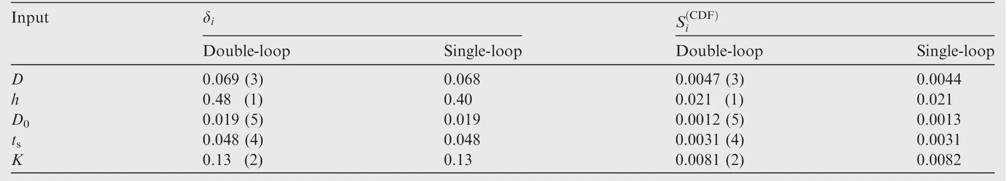
Table 2 Importance measures of inputs for riveting example.

According to Property III shown in Section 3.3,we define two ratio functions for RIMPDF and RIMCDF as

The ratio functions,Hi（q1，q2）andKi（q1，q2）,can reflects the reductions of the two moment-independent importance measures by reducing the range ofXifrom （-∞，+∞）to［xi，1，xi，2］(noting thatTake the most important input,h,for example.The ratio functions of RIMPDF and RIMCDF ofhare shown in Fig.4.In the 3D plots,the lower the values ofHh（q1，q2）andKh（q1，q2）are,the more reductions of the contribution ofhto the output distribution will be obtained by reducing its range.Similar discussions can be performed on the other inputs,and they are not listed here to save space.Despite of the difference between the absolute values in Figs.4(a)and(b),the two plots exhibit a similar trend,which is possibly due to the fact that PDF is highly related to CDF.In Ref.,20Tarantola et al.derived several interesting observations for the 3D plots of variance ratio functions.In a similar manner,the ratio functions of RIMPDF and RIMCDF can be interpreted as follows:

(1)The contribution to the PDF or CDF of the output can be estimated for any region ［q1，q2］of an input.

(2)The counter-diagonal line of the 3D plot of Hi（q1，q2）or Ki（q1，q2）represents the ratio function by the symmetric reduction of the range from both sides of the range,i.e.,from the quantile interval ［0，1］to ［q，1-q］with 0≤q≤0.5.The one-dimensional ratio functions of RIMPDF and RIMCDF for all the inputs are shown in Fig.5

(3)The diagonal lines of the 3D plots represent the situation q1=q2=qorthederivativesofRIMPDF and RIMCDF,i.e.,Hi（q，q）=d（RIMPDFXi（q））/dqand Ki（q，q）=d（RIMCDFXi（q））/dq.It measures the effects on the moment-independent importance measures by fixing an input at quantileq.The functions Hi（q，q）and Ki（q，q）for all the inputs are illustrated in Fig.6.

In Fig.5,conclusions can be drawn that the contributions of the inputs to the output PDF and CDF decrease with the symmetric reduction of the input ranges.Quantitative information is also available.In Fig.5(a),it can be found thatHh（0.2，1-0.2）=0.8,which indicates that by reducing the distribution range ofhfrom the quantile interval ［0，1］to［0.2，0.8］,the contribution ofhto the output PDF can be reduced by 20%. Meanwhile, in Fig.5(b),we seeKh（0.2，1-0.2）=0.65,which indicates that the contribution ofhto the output CDF can be reduced by 35%by reducing the range ofhfrom the quantile interval ［0，1］to ［0.2，0.8］.The contribution can be further reduced if continuing to reduce the range ofh.Similar studies can be conducted on the other inputs.Furthermore,Fig.5 both show that for each input,the tail area is more concerned with the output uncertainty than the center area,since the one-dimensional plots change more steeply in the tail area.

Fig.6 can offer information about how much the contribution of an input to the output uncertainty can be changed by fixing the input at different values ofq.As declared above,the one-dimensional plots in Fig.6 are derivatives of the corresponding RIMPDF and RIMCDF.Taking the inputhfor example,in Fig.6(a),it shows thatHh（0.5，0.5）=0.75,which indicates that its contribution to the output PDF can be reduced by as much as 25%if we f i xhat its median value.An interesting phenomenon is noticed here,i.e.,its contribution to the output uncertainty tends to increase when fixing an input near the tail area.These conclusions are rather informative for analysts when uncertainty of the output needs to be controlled.

4.2.Example 2:A ten-bar structure

Consider a ten-bar structure with 15 input variables,which is depicted in Fig.7.The length and sectional area of horizontal and vertical bars are denoted asLandAi（i=1，2，...，6）,while the length and sectional area of diagonal bars are■■2■LandAi（i=7，8，9，10）.The elastic modulus of all bars is denoted asE.P1,P2，andP3are the external loads.In this problem,the 15 input variables are denoted asX= ［Ai（i=1，2，...，10），L，P1，P2，P3，E］,with the distribution information listed in Table 3.Taking the perpendicular displacement of Node 2,d,not exceeding 0.004 m as the constraint condition,the model can be established as

wheredis an implicit function of the inputs.

Table 3 Distribution information of inputs for ten-bar example.

The model in this example needs to be evaluated by calling ANSYS codes,and thus the computation process will be timeconsuming if the double-loop method is used.The results of the two moment-independent importance measures,δiand,are obtained by the single-loop method and presented in Fig.8.

The results in Fig.8 can reflects the contributions of the inputs to the output uncertainty from the viewpoint of probabilistic distribution.The inputs can be ranked according to the importance measures in a descending order asL,E,P1,P2,A1,A3,A7,A8,P3,A9,A5,A10,A4,A6,andA2.In fact,the contributions byA2,A4,A5,A6,andA10are so tiny that they can almost be neglected compared to the rest.The importance analysis can thus provide helpful advice for the improvement of the model,and dig out some underlying information associated with the inputs.

We now take a further step to perform regional importance analysis on the three most important inputs,L,E,andP1.As in this example,the importance ranking based on δiis the same as that based on,we will only study the RIMPDF of the three inputs.The RIMPDF plots for the inputsL,E,andP1are presented in Fig.9,where the plots show a similar trend.Taking the inputLfor example,its contribution to the output PDF turns out to be uneven through its distribution range.The RIMPDF plot is above the diagonal in the left tail ofL,which means that its contribution to the output PDF is higher than the average,and its contribution is lower than the average in the right tail as the plot goes below the diagonal in this region.Similar conclusions can be drawn for the inputsEandP1.

As pointed out in the last example,the ratio functions,Hi（q1，q2）andKi（q1，q2）,can represent the ratios of the moment-independent importance measures before and after the input range is reduced from the quantile interval ［0，1］to［q1，q2］.Here,Hi（q1，q2）is plotted for the top three important inputs,L,E,andP1,in the formulation of the 3D plots by Fig.10.It is noticed that the 3D plots are similar to each other,which indicates that the information obtained by performing the regional importance analysis for one input possibly holds true for another.Again,in the 3D plots,the lower the value ofHi（q1，q2）is,the more reduction of input contribution is obtained by reducing the input range.

The counter-diagonal lines corresponding to the 3D plots in Fig.10 are plotted in Fig.11.These lines reflects the reductions of the contributions of the inputsL,E,andP1to the output PDF by symmetrically reducing the ranges from both sides of the ranges.It shows that the counter-diagonal line of the inputLalmost coincides with that ofE.Taking the inputP1for example,we seeHP1（0.25，1-0.25）=0.5,which indicates that by reducing the distribution range ofP1from the quantile interval［0，1］to ［0.25，0.75］,the contribution ofP1to the output PDF can be reduced by as much as 50%.Meanwhile,the diagonal lines corresponding to the 3D plots in Fig.10 are plotted in Fig.12,which can reflects how much the contribution of an input to the output uncertainty can be changed by fixing the input at different values ofq.As declared in last example,the diagonal line can be mathematically interpreted as the derivative of the RIMPDF.

5.Conclusions

Enlightened by CSM and CSV,the idea of regional analysis is extended to the moment-independent importance analysis in this work.Two new definitions,RIMPDF and RIMCDF,aiming to evaluate the contributions of specific regions of an input to the output PDF and CDF,are introduced.The properties are discussed,as well as the corresponding computational strategies.By performing the regional moment-independent importance analysis,information concerning how the regions inside the inputs affect the whole output distribution can be obtained.Such information is helpful for analysts to control the output uncertainty,as PDF and CDF are more sufficient to describe the uncertainty than solely depending on the mean or variance.Meanwhile,RIMPDF and RIMCDF can be obtained with the same samples used to estimate δiand,and thus they can be viewed as byproducts of the standard moment-independent importance analysis,without a need of extra model evaluations.The idea of RIMPDF and RIMCDF provides not a substitution but a viable supplement to sensitivity analysis.Discussions on applying RIMPDF and RIMCDF in two engineering cases demonstrate that the regional moment-independent importance analysis can add more information concerning the contributions of model inputs.

Acknowledgements

This study was supported by the National Natural Science Foundation of China(No.NSFC51608446)and the Fundamental Research Fund for Central Universities of China(No.3102016ZY015).

1.Saltelli A.Sensitivity analysis for importance assessment.Risk Anal2002;22:579–90.

2.Rahman S.Stochastic sensitivity analysis by dimensional and score functions.Probabilist Eng Mech2009;24:278–87.

3.Zhou C,Lu Z,Li L,Feng J,Wang B.A new algorithm for variance based importance analysis of models with correlated inputs.Appl Math Model2013;37:864–75.

4.Borgonovo E,Plischke E.Sensitivity analysis:a review of recent advances.Eur J Oper Res2016;248:869–87.

5.Saltelli A,Marivoet J.Non-parametric statistics in sensitivity analysis for model output:A comparison of selected techniques.Reliab Eng Syst Safe1990;28:229–53.

6.Iman RL,Johnson ME,Watson Jr CC.Sensitivity analysis for computer model projections of hurricane losses.Risk Anal2005;25:1277–97.

7.Sobol IM.Global sensitivity indices for nonlinear mathematical models and their Monte Carlo estimates.Math Comput Simul2001;55:271–80.

8.Rabitz H,Alis OF.General foundations of high-dimensional model representations.J Math Chem1999;25:197–233.

9.Saltelli A,Tarantola S,Campolongo F.Sensitivity analysis as an ingredient of modelling.Stat Sci2000;19:377–95.

10.Frey CH,Patil SR.Identif i cation and review of sensitivity analysis methods.Risk Anal2002;22:553–71.

11.Park CK,Ahn KI.A new approach for measuring uncertainty importance and distributional sensitivity in probabilistic safety assessment.Reliab Eng Syst Safe1994;46:253–61.

12.Chun MH,Han SJ,Tak NI.An uncertainty importance measure using a distance metric for the change in a cumulative distribution function.Reliab Eng Syst Safe2000;70:313–21.

13.Borgonovo E.A new uncertainty importance measure.Reliab Eng Syst Safe2007;92:771–84.

14.Borgonovo E.Measuring uncertainty importance:investigation and comparison of alternative approaches.RiskAnal2006;26:1349–61.

15.Liu Q,Homma T.A new importance measure for sensitivity analysis.J Nucl Sci Technol2010;47:53–61.

16.Castaings W,Borgonovo E,Morris MD,Tarantola S.Sampling strategies in density-based sensitivity analysis.Environ Model Softw2012;38:13–26.

17.Millwater M,Singh G,Cortina M.Development of localized probabilistic sensitivity method to determine random variable regional importance.Reliab Eng Syst Safe2012;107:3–15.

18.Sinclair J.Response to the PSACOIN Level S exercise.PSACOIN Level S intercomparison.Pairs:Nuclear Energy Agency,Organisation for Economic Co-operation and Development;1993.

19.Bolado-Lavin R,Castaings W,Tarantola S.Contribution to the sample mean plot for graphical and numerical sensitivity analysis.Reliab Eng Syst Safe2009;94:1041–9.

20.Tarantola S,Kopustinskas V,Bolado-Lavin R,Kaliatka A,Uspuras E,Vaisnoras M.Sensitivity analysis using contribution to sample variance plot:Application to a water hammer model.Reliab Eng Syst Safe2012;99:62–73.

21.Wei P,Lu Z,Wu D,Zhou C.Moment-independent regional sensitivity analysis:Application to an environmental model.Environ Model Softw2013;47:55–63.

22.Plischke E,Borgonovo E,Smith CL.Global sensitivity measures from given data.Eur J Oper Res2013;226:536–50.

23.Botev ZI,Grotowski JF,Kroese DP.Kernel density estimation via diffusion.Ann Stat2010;38:2916–57.

24.Wei P,Lu Z,Yuan X.Monte Carlo simulation for momentindependent sensitivity analysis.ReliabEngSystSafe2013;110:60–7.

25.Borgonovo E,Hazen GB,Plischke E.A common rationale for global sensitivity measures and their estimation.Risk Anal2016;36(10):1871–95.

26.Yun W,Lu Z,Jiang X,Liu S.An efficient method for estimating global sensitivity indices.Int J Numer Meth Eng2016;108(11):1275–89.

27.Rahman S.A surrogate for density-based global sensitivity analysis.Reliab Eng Syst Safe2016;155:224–35.

28.Cheraghi SH.Effect of variations in the riveting process on the quality of riveted joints.IntJAdvManufTechnol2008;39:1144–55.

29.Mu W,Li Y,Zhang K,Cheng H.Mathematical modeling and simulation analysis of flush rivet pressing force.J Northwest Polytech Univ2010;28:742–7[Chinese].

22 March 2016;revised 13 December 2016;accepted 2 March 2017