A GPU accelerated finite volume coastal ocean model*

Xu-dong Zhao (赵旭东), Shu-xiu Liang (梁书秀), Zhao-chen Sun (孙昭晨), Xi-zeng Zhao (赵西增), Jia-wen Sun (孙家文), Zhong-bo Liu (刘忠波)

1.State Key Laboratory of Coastal and Offshore Engineering, Dalian University of Technology, Dalian 116023, China, E-mail: zhaoxvdong@dlut.edu.cn

2.Ocean College, Zhejiang University, Zhoushan 316021, China

3.National Marine Environmental Monitoring Center, State Oceanic Administration, Dalian 116023, China

4.Transportation Management College, Dalian Maritime University, Dalian 116026, China

A GPU accelerated finite volume coastal ocean model*

Xu-dong Zhao (赵旭东)1, Shu-xiu Liang (梁书秀)1, Zhao-chen Sun (孙昭晨)1, Xi-zeng Zhao (赵西增)2, Jia-wen Sun (孙家文)3, Zhong-bo Liu (刘忠波)4

1.State Key Laboratory of Coastal and Offshore Engineering, Dalian University of Technology, Dalian 116023, China, E-mail: zhaoxvdong@dlut.edu.cn

2.Ocean College, Zhejiang University, Zhoushan 316021, China

3.National Marine Environmental Monitoring Center, State Oceanic Administration, Dalian 116023, China

4.Transportation Management College, Dalian Maritime University, Dalian 116026, China

With the unstructured grid, the Finite Volume Coastal Ocean Model (FVCOM) is converted from its original FORTRAN code to a Compute Unified Device Architecture (CUDA) C code, and optimized on the Graphic Processor Unit (GPU). The proposed GPU-FVCOM is tested against analytical solutions for two standard cases in a rectangular basin, a tide induced flow and a wind induced circulation. It is then applied to the Ningbo’s coastal water area to simulate the tidal motion and analyze the flow field and the vertical tide velocity structure. The simulation results agree with the measured data quite well. The accelerated performance of the proposed 3-D model reaches 30 times of that of a single thread program, and the GPU-FVCOM implemented on a Tesla k20 device is faster than on a workstation with 20 CPU cores, which shows that the GPU-FVCOM is efficient for solving large scale sea area and high resolution engineering problems.

Graphic Processor Unit (GPU), 3-D ocean model, unstructured grid, finite volume coastal ocean model (FVCOM)

Introduction

The parallel computational schemes and the large scale, high resolution climate and ocean simulation models see a rapid development. The traditional CPU parallel algorithms for large scale ocean simulations are generally performed by the domain decomposition, where the domain is divided into many sub-domains with each sub-domain dealt by a different processor using distributed or shared memory computing. These parallel computational ocean models are mostly based on the Message Passing Interface (MPI) library, requiring High Performance Computing (HPC) clusters to realize the high computational capacity. Therefore, the high performance is difficult to achieve withoutaccess to HPC computers.

In recent years, microprocessors based on a single Central Processing Unit (CPU) have greatly enhanced the performance and reduced the cost in computer applications[1,2]. However, the increase of the CPU computing capacity is limited due to heating and transistor density limitations. However, the CPU is not the only processing unit in the computer system. The Graphic Processor Unit (GPU) is initially used for rendering images, but is also a highly parallel device[3]. The GPU’s main task remains rendering video games, which is achieved by a fine gained parallelism for pixels rendered with a large number of microprocessors. Multiple threaded processors, and particularly, the GPUs, have enhanced the floating point performance since 2003[4]. NVIDIA provided a GPU computing Software Development Kit (SDK) in 2006 that extended the C programming language to use GPUs for general purpose computing. The ratio between multiple core GPUs and CPUs in the floating point calculation throughput is approximately 10:1 in 2009, i.e., the multiple core GPUs could reach 1 teraflops (1 000 gigaflops), while CPUs could onlyreach 100 gigaflops. Figure 1 shows that with the GPU Computing Accelerator, NVIDIA Tesla K40M, the double precision floating point performance has now reached 1.68 Tflops.

Fig.1(a) Floating point operation performance

Fig.1(b) Memory bandwidth for the CPU and GPU

A number of programs and applications have been ported to the GPU, such as the lattice Boltzmann method[5], Ansys[6], and DHI MIKE. The use of the GPU devices was also explored for ocean and atmosphere predictions[7,8]. Michalakes and Vachharajani[9]proposed a Compute Unified Device Architecture (CUDA) C based weather prediction model. They achieved a twenty-fold speedup (by using NVIDIA 8800 GTX) compared to a single-thread Fortran program running on a 2.8 GHz Pentium CPU[9]. Most existing climate and ocean models are only accelerated for specific loops using the open accelerator application program interface (OpenACC-API) or CUDA Fortran, therefore these GPU accelerated models have achieved limited speedup. Horn implemented the GPU to a moist fully compressible atmospheric model[10]. Xu et al.[11]developed the Princeton Ocean Model POM.gpu v1.0, a full GPU solution based on MPI version of the Princeton Ocean Model (mpiPOM). POM.gpu v1.0 with four GPU devices can match the performance of the mpiPOM with 408 standard CPU cores. However, they were unable to resolve the complex irregular geometries of tidal creeks in an estuarine application[12]. Keller et al.[13]developed a GPU accelerated MIKE21 to solve 2-D hydrodynamics problems, and the latest DHI MIKE (2016) supports the GPU based 3-D hydrodynamic parallel computing.

The objective of this work is to reduce the computation time for the unstructured grid, Finite Volume Coastal Ocean Model (FVCOM) with a CUDA C parallel algorithm. The CUDA is a minimal extension of the C and C++ programming languages, and allows a program to be generated and executed on GPUs.

With the FVCOM parallel version, we demonstrate how to develop a GPU based ocean model (GPU-FVCOM) that runs efficiently on a professional GPU. The Fortran FVCOM is first converted to the CUDA C, and optimized for the GPU to further improve the performance.

In this work, the GPU-FVCOM performance is tested for two standard cases in rectangular basins with different grid numbers and devices, and then applied to the Ningbo coastal region. Particular attention is paid to the tidal current behavior, including the current velocity and the time history of sea levels.

1. Unstructured grid, finite volume coastal ocean model

The FVCOM is a prognostic, unstructured grid, finite volume, free surface, 3-D primitive equation coastal ocean circulation model jointly developed by UMASSD-WHOI. To solve the large scale sea area and high grid density problem, the METIS partitioning libraries are used to decompose the domain, and to implement the explicit Single Program Multiple Data (SPMD) parallelization method to the FVCOM[14]. The FVCOM has also been used in a wide range of engineering problems[15-19].

In the horizontal direction, the spatial derivatives are computed using the cell vertex and cell centroid (CV-CC) multigrid finite volume scheme. In the vertical direction, the FVCOM supports the terrain following sigma coordinates. The 3-D governing equations can be expressed as:

and

wheretrepresents the time,Dis the water depth,ξdenotes the surface elevation,xandyare the Cartesian coordinates,σis the sigma coordinate,u,vandwrepresent the velocity components in thex,yandσdirections,gis the coefficient of gravity,fis the coefficient of Coriolis force, andAmandKmrepresent the horizontal and vertical diffusion coefficients, respectively.

The FVCOM uses the time splitting scheme to separate the 2-D (external mode) from the 3-D (internal mode) momentum equations. The external mode calculation updates the surface elevation and the vertically averaged velocities. The internal mode calculation updates the velocity, the temperature, the salinity, the suspended sediment concentration, and the turbulence quantities.

The momentum and continuity equations for the internal mode are integrated numerically using the explicit Euler time stepping scheme, and those for the external mode are integrated using a modified second order Runge-Kutta scheme

wheredenotes the residual,Ωis the area of the control volume element, ΔtErepresents the external time step, the superscriptsnandn+1 denote the external time levels, andkdenotes the Runge-Kutta level. Since the spatial accuracy of the discretization is of the second order, the simplified Runge-Kutta scheme is sufficient.

The external and the internal modules are the most computationally intensive kernels. In this work, the modified Mellor and Yamada level 2.5 turbulent closure scheme is implemented for the vertical and horizontal mixing, respectively.

The FVCOM is a multi-function ocean model, and the source code is very large. The GPU-FVCOM implements only the 3-D hydrodynamics, the temperature, the salinity, and the sediment transport. A full port of the FVCOM to the GPU-FVCOM remains to be done in the future research.

2. Algorithm development

In contrast to the traditional parallel programs executed on the CPU, the GPU is specialized for intensive, highly parallelizable problems. Many more transistors are designated for data processing rather than data caching and flow control[20]. As many threads should be assigned in parallel as possible, where each thread executes a specific computing task.

The CUDA allows the user convenient programming and execution of data level parallel programs on the GPU. The data parallel processing maps the data elements to the parallel processing threads. Each thread processes data element rather than the loop computing. The GPU support is now available for the MATLAB and the CUDA development becomes much easier with C/C++/Fortran and Python, however, some new features and math libraries only support the CUDA C language.

In this work, a massively parallel GPU version of the FVCOM is developed based on the CUDA C. In the GPU-FVCOM, the CPU is only used to initialize variables, output results, and activate device subroutines executed on the GPU. The overall and optimization strategies for the GPU-FVCOM are introduced in the following sections.

2.1 Preliminary optimization

The first stage of the GPU-FVCOM development involves the following method to realize data level parallelism without optimization.

Figure 2 illustrates the code structure of the GPU-FVCOM. The major difference between the FVCOM and the GPU-FVCOM is that the CPU is only used for initializing the relevant arrays and providing the output. The GPU executes all model computing processes, and the data is only sent to the host for the file output at user-specified time steps.

Fig.2 Flowchart of GPU-FVCOM processing

(1) Data stored in the global memory and repeatedly accessed in the GPU threads are replaced by temporary variables stored in the local register memory. The register memory in the GPU threads can be accessed faster than the global memory. Figure 3 shows that this approach improves the GPU-FVCOM performance by 20%.

Fig.3 Speedup ratio of kernel function with/without utilizing register compared with sequential program

Fig.4 Sample code without/with atomic memory operations

Fig.5 Loop fusion and original method

(2) The GPU takes up a large number of threads simultaneously. While solving the momentum equations, the GPU-FVCOM loops with the element edges. With this approach, two or more threads attempting to access the same data will cause memory operation errors and return a wrong answer. To avoid memory access conflicts, atomic memory operations are implemented on the GPU to ensure only one thread at a time performs the read-modify-write operation, as shown in Fig.4. Implementing this process reduces the execution time of the kernel function by almost 50%.

Fig.6 Ratio of original algorithm to loop fusion method execution times for numbers of different horizontal grids (line type) and sigma layers (x-axis)

(3) The loop fusion is optimized by merging several sequential loops with the same cycle times into one loop. The loop fusion is an effective and simple method to reduce the global memory access and to transfer the global memory to registers for repeated use of the same data. The GPU reads from the global memory and transfers the value to the register memory. Figure 5 shows the different execution processing of the CUDA parallel program with and without using the loop fusion method. With the loop fusion method, we fuse the sequential loops into one kernel function and use the register variables to reduce the global memory access latency.

With this method, the GPU-FVCOM computational performance is significantly improved. Figure 6 shows that the speedup ratios (the ratio of the original algorithm execution time to the loop fusion method execution time) for different horizontal grid numbers increase with the increase of the number of sigma levels.

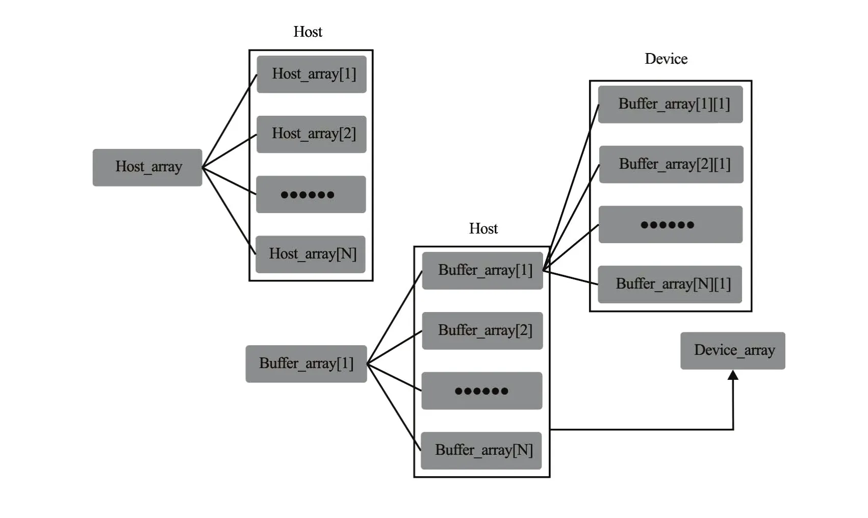
Fig.7 Passing a 2-D array from host memory to device memory

Fig.8 The relationship ofσlayer distribution and threads assignment

Thus, the execution speed is improved by 70%, if there are adequate horizontal grids and sigma levels.

2.2 Special optimization

(1) Implementation of multidimensional array data. Since the GPU and CPU memories are independent,the CUDA cannot simply use the “cudaMemcpy”to transfer the multidimensional array variables (dynamically allocated) between the CPU and the GPU. In the CUDA API libraries, the“cudamalloc” function is only used to allocate a linear memory on the device and returns a pointer to the allocated graphic memory, the “cudaMemcpy” copies the data from the memory area pointed to by the source memory pointer to the memory area pointed to by the destination memory pointer. Figure 7 shows how the novel array passing method is implemented in this work. Consequently, the multidimensional arrays can be directly accessed by the kernel function.

Fig.9 Kernel scaling on stream multiprocessors

Table 1 GPU utilization for different numbers of threads per block

(2) Optimization with height dependence release. In some 3-D kernel functions,kcomponents of the sigma layers are not independent when solving the vertical diffusion term of the momentum and turbulence equations. The GPU-FVCOM uses akcomponent loop of the sigma layer in the kernel function to reduce the shared data access, and in each thread,kcomponents are computed. For the horizontal advection term, thekth component does not depend on other layer components. The GPU grid size is divided intoklevels, and in each thread, one component is computed. The kernel functions are shown in Fig.8.

The height dependence is an effective method to hide the global memory access latency. It stores scalar variables in registers for the data reuse. The execution time is thus reduced by 10%-50%.

(1) Optimization with block size. The streaming multiprocessors (SMs) are the part of the GPU that runs the CUDA kernel functions. The occupancy of each SM is limited by the thread number per block, register usage, and shared memory usage. As shown in Fig.9, the threads in each block are executed by the same SM. Each SM splits its own blocks into warps (currently 32 threads per warp). The GPU device needs more than one thread per core to hide the global memory latency and run with high performance. To fully use the computational capability of each SM, the thread number in each block should be a multiple of the warp size.

The Tesla K20x card supports up to 64 active warps per streaming multiprocessor, and contains 14 multiprocessors and 2 688 cores (192 stream processors per multiprocessor). The Single Instruction, Multiple Thread (SIMT) execution model is implemented in the CUDA architecture. The GPU utilization for different computing capability for different threads per block are shown in Table 1. The only case that obtains 100 percent utilization across all generations of the GPU device is 256 threads per block. Several tests are conducted, and the experimental results are consistent with Table 1. Therefore, to en-sure the maximum GPU utilization, we assign 256 threads per block.

3. Numerical scheme verification

Two test cases are selected to analyze the GPU-FVCOM computing efficiency and accuracy. Both cases are run on a variety of GPU devices, and the speedup ratios are approximately the same in each case. Thus, for space considerations only the speedup ratios for the first case with different devices, parallel tools, and grid numbers are presented.

3.1 Verification of 2-D and 3-D M2tidal induced current circulation

The GPU-FVCOM is applied to the tide induced circulation in a rectangular basin with a length of 3.4 km, a width of 1.6 km and a depth of 10 m. The geometry and the horizontal meshes are shown in Fig.10.

Fig.10 Horizontal meshes for 2-D and 3-D tidal induced circulation

AnM2tide with the maximum amplitude of 1 m at the open boundary is used as the free surface water elevation. In this case, the Coriolis force coefficient isf=0, and the analytical solution is

and

whereAis the tidal amplitude,ω=2π/Tis the angular frequency,his the water depth,xis the distance between the verified point to the left solid boundary,Tis theM2tidal period,ξis the free surface elevation, anduis the longitudinal component of the depth-average horizontal velocity. The numerical simulation parameters are shown in Table 2.

Figure 11 compares the computed free surface elevation and the depth-averaged velocities at the verified point with the analytical solutions. The maximumwater surface elevations are in agreement within a margin of 3.5% and the maximumu-velocity components are in agreement within a margin of 4.2%.

Table 2 Model parameters for the tidal induced test case

Fig.11 Analytical and computed of the basin

3.2 Verification of 3-D wind induced circulation

This experiment validates the proposed model’s capability in simulating the wind induced circulation in a closed rectangular basin, as shown in Fig.12. Using the no-slip condition at the channel bed, the uniform and steady state analytical solutions for the horizontal velocity component in a well-mixed channel with a known constant vertical eddy viscosity coefficient is obtained aswhereuis the horizontal velocity component inx-direction,his the water depth,ξis the free surface elevation above the initial water elevation,is the eddy viscosity coefficient in the vertical direction,is thexcomponent of the surface wind stress, andρis the water density.

Fig.12 Horizontal meshes for wind induced circulation

Table 3 Model parameters for the wind induced test case

Fig.13 Analytical and computedx-component of horizontal velocity profiles in vertical direction at the center of the rectangular basin

Bottom stress is

A rectangular basin with a length of 2.0 km and a width of 0.8 km is used, with related parameters as shown in Table 3.

The convergence results are obtained from a cold start after the program runs for 10 internal time steps. To avoid the influence of the reflection from the solid boundary, the central point of the rectangular basin is chosen as the verification point, and the computed horizontal velocity along the vertical profile is compared with the analytical solution, as shown in Fig.13.

3.3 Comparisons of computational performance on variety of devices

Computational performance of sequential programming, the MPI parallel code, and the GPU code for the ocean model is compared for three different GPU devices, shown in Table 4. The simulations are run for five horizontal meshes: 1 020, 4 080, 16 320, 65 280 and 261 120, which are implemented on the 3-D GPU-FVCOM. To fully utilize the GPU performance, the kernel function is used to solve the advection diffusion equation of each element.

Table 4 Hardware device versions

Figure 14 compares the speedup for 3-D simulations for a variety of horizontal meshes and devices in the tidal induced case. The speedup ratio is the computational time for a single thread program divided by that for a parallel program.

Fig.14 Speedup of 3-D simulations for a variety of meshes and devices in the tidal induced case

When the number of the grid nodes is less than 16 320, the 2-D and 3-D GPU-FVCOM speedup ratios are less than that of the MPI parallel code. However, when the number of the grid nodes reaches 65 280, the 3-D GPU-FVCOM speedup ratio exceeds that of the MPI parallel code.

Speedup ratio is more than 31 for the 3-D simulation with the 261120 nodes grid. For a low horizontal resolution, the GPU-FVCOM speedup running on the Tesla K20M is less than that of the MPI parallel program running on a 32 thread HPC cluster.However, the speedup of the MPI parallel with 32 threads decreases slightly when the number of the grid nodes approaches 261120, whereas the GPU-FVCOM speedup is still in increase. Thus, with the grid sizes in the trial run, the Tesla K20M performance is not fully exploited. Further increasing the number of threads (with larger grid density) will produce larger speedups for professional GPU computing devices.

Fig.15 Simulation time for each data update with different sigma levels and horizontal meshes in the tidal induced case executed on Tesla K20Xm

Figure 15 compares the execution time for each data update with different sigma levels and horizontal meshes in the tidal induced case executed on the Tesla K20Xm. The 5-sigma-layer execution time and the 50-sigma-layer execution time are 2-4 times and 5-19 times of that of the 2-D model. Extrapolating from these results, the 2-D model performance is 28 MCUPS (Million Cells Update Per Second).

Therefore, the GPU power can be gradually exploited by increasing the grid resolution and sigma levels. When the grid vertices exceed approximately 65 000, the GPU-FVCOM computing efficiency exceeds that of a 32 thread MPI parallel ocean model. Thus, the GPU-FVCOM has a significant potential for large scale domain and high resolution computations while maintaining the practical computing time.

4. Application to Ningbo’s coastal waters

4.1 Model configuration and verification

The GPU-FVCOM is applied to simulate the flow field of the Ningbo water area, which has the most complicated coastline and topography in China.

The computational domain covers all Ningbo’s coastline and neighboring islands, with more than 174 000 triangle meshes. The horizontal computational domain is shown in Fig.16, covering an area of 200×220 km. The length of the element side varies from 150 m for complex coastlines to 3 500 m for offshore areas, and 11 sigma levels are adopted for the depth.

Fig.17 Simulated and measured tidal elevations at station T1

Fig.18 Simulated and measured surface tidal currents at station 1#

The GPU-FVCOM verification is made by comparing simulated and measured data. The data come from measurements over the period from 30 June to 1 July, 2009. Measurement stations are shown in Fig.16, including 7 tidal elevation stations (T1-T7) and 8 tidalcurrent stations (1#-8#). In this work, T1 and 1# are chosen as the representative stations.

Figure 17 compares the simulated and observed water surface elevations at station T1. The simulated and measured data show good agreement, with the magnitude and the phase of the free surface water elevation being well matched.

Figure 18 compares the simulated and observed tide induced currents at stations 1#. The simulated and observed currents show good agreement, with the magnitude and the phase favorably matched.

4.2 Flow field characteristics

Figure 19 shows the surface flow field at the time of floor tide. The simulated result shows that the tide flows southeast along the Ningbo and Zhoushan coastlines. The tide flows through Nan Jiushan, then into the Xiangshan Bay and the Hangzhou Bay. The tide direction is along the coastline of the Hangzhou Bay. The average flood tide direction is between 230oand 300o. The flow at the north of the Hangzhou Bay is affected by the flood tides, and the water flux is net input.

The current speed along the northern coastline is larger than that along the southern shore at the flood tide. After the tide flows into the Xiangshan Bay, the impact of the topography and the reflection of the land boundary gradually turns the tide from a progressive tidal wave to a standing wave, with the tidal range gradually increasing from the entrance to the inner bay.

Overally, the results show that the GPU-FVCOM can simulate the flow field of the Ningbo’s water area satisfactorily.

4.3 Computational performance for Ningboʼs coastal waters

Figure 20 shows the GPU-FVCOM speedup for different GPU devices. Speedup ratios are similar for the same grid number. The GPU-FVCOM executed on the GTX 460 produces a speedup approximately 13 times of that of the 3-D single thread program. The Tesla K20Xm GPU provides a speedup of 27. Hence, the GPU-FVCOM can yield a powerful computational performance to solve arbitrary ocean circulation topographies, and the GPU accelerated FVCOM is significantly faster.

Fig.20 Speedup ratio for different GPU devices for Ningbo coastal water simulation

5. Conclusions

A GPU based parallelized version of the FVCOM is developed and optimized for the GPU parallel implementation. The speedup for the 3-D ocean model is impressive: up to 30 times speedup with high grid densities.

Two classic experiments are performed to validate the accuracy of the proposed GPU-FVCOM. The 2-D GPU-FVCOM achieves 27 times speedup when the number of grid vertices exceeds 2.6×104. Under the same conditions, the GPU-FVCOM speedup is superior to a 32 thread MPI parallel program running on a cluster. The 3-D GPU-FVCOM achieves 31 times speedup. Even using a laptop graphic card K780M, the computational performance of the 3-D GPU-FVCOM is slightly superior to a 32 thread MPI parallel program running on a high performance cluster.

The GPU-FVCOM is applied to simulate the tidal motion of the Ningbo coastal water with a complicated coastline. The simulated results for the surface elevations and the current velocity are in goodagreement with the measured data. The simulated velocity shows the current speed differences between the surface and bottom layers. A large quantity of water flows into the Xiangshan Bay and the Hangzhou Bay. After flowing into the Xiangshan Bay, the impact of the topography and the reflection of the land boundary gradually turns the progressive tidal wave to a standing wave. The speedup of the GPU-FVCOM varies for different GPU devices. The 3-D GPUFVCOM model retains a high speedup, and the computational performance is significantly superior to that of a MPI parallel program executed on a high performance workstation with 32 CPU cores.

The GPU-FVCOM has a tremendous potential to solve massively parallel computational problems, and may be well suited and widely applied for high resolution hydrodynamic and mass transport problems. Future work will be concentrated on the MPI and multiple GPU hybrid accelerated versions of the GPUFVCOM.

[1] Ruetsch G., Fatica M. CUDA Fortran for scientists and engineers: Best practices for efficient CUDA fortran programming [M]. Burlington, USA: Morgan Kaufmann, 2013.

[2] Wilt N. The CUDA handbook: A comprehensive guide to GPU programming [M]. Boston, USA: Addison-Wesley Professional, 2013.

[3] Chen T. Q., Zhang Q. H. GPU acceleration of a nonhydrostatic model for the internal solitary waves simulation [J].Journal of Hydrodynamics, 2013, 25(3): 362-369.

[4] Kirk D. B., Hwu W. M. Programming massively parallel processors: A hands-on approach [M]. Burlington, USA: Morgan Kaufmann, 2012.

[5] Bailey P., Myre J., Walsh S. D. et al. Accelerating lattice Boltzmann fluid flow simulations using graphics processors [C].The 38th international conference on parallel processing.Vienna, Austria, 2009.

[6] Krawezik G. P., Poole G. Accelerating the ANSYS direct sparse solver with GPUs [C].Symposium on Application Accelerators in High Performance Computing. Champaign, USA, 2009.

[7] Huang M., Mielikainen J., Huang B. et al. Development of efficient GPU parallelization of WRF Yonsei University planetary boundary layer scheme [J].Geoscientific Model Development, 2015, 8(9): 2977-2990.

[8] Lacasta A., Morales-Hernández M., Murillo J. et al. An optimized GPU implementation of a 2D free surface simulation model on unstructured meshes [J].Advances in Engineering Software, 2014, 78: 1-15.

[9] Michalakes J., Vachharajani M. GPU acceleration of numerical weather prediction [J].Parallel Processing Letters, 2008, 18(4): 531-548.

[10] Horn S. ASAMgpu V1. 0-a moist fully compressible atmospheric model using graphics processing units (GPUs) [J].Geoscientific Model Development, 2011, 4(2): 345-353.

[11] Xu S., Huang X., Oey L. Y. et al. POM.gpu-v1.0: A GPU-based princeton ocean model [J].Geoscientific Model Development, 2015, 8(9): 2815-2827.

[12] Chen C., Huang H., Beardsley R. C. et al. A finite volume numerical approach for coastal ocean circulation studies: Comparisons with finite difference models [J].Journal of Geophysical Research: Oceans, 2007,112(C3): 83-87.

[13] Keller R., Kramer D., Weiss J. P. Facing the Multicore-Challenge III [M]. Berlin, Heidelberg, Germany: Springer 2013, 129-130.

[14] Cowles G. W. Parallelization of the FVCOM coastal ocean model [J].International Journal of High Performance Computing Applications.2008, 22(2): 177-193.

[15] Bai X., Wang J., Schwab D. J. et al. Modeling 1993- 2008 climatology of seasonal general circulation and thermal structure in the Great Lakes using FVCOM [J].Ocean Modelling, 2013, 65(1): 40-63.

[16] Zhang A., Wei E. Delaware River and Bay hydrodynamic simulation with FVCOM [C].Proceedings of the 10th International Conference on Estuarine and Coastal Modeling, ASCE. Newport, USA. 2008.

[17] Chen C., Huang H., Beardsley R. C. et al. Tidal dynamics in the Gulf of Maine and New England Shelf: An application of FVCOM [J].Journal of Geophysical Research: Oceans, 2011, 116(C12): 12010.

[18] Liang S. X., Han S. L., Sun Z. C. et al. Lagrangian methods for water transport processes in a long-narrow bay-Xiangshan Bay, China [J].Journal of Hydrodynamics, 2014, 26(4): 558-567.

[19] CHEN Y. Y., LIU Q. Q. Numerical study of hydrodynamic process in Chaohu Lake [J].Journal of Hydrodynamics, 2015, 27(5): 720-729.

[20] Cook S. CUDA programming: a developerʼs guide to parallel computing with GPUs [M]. Burlington, USA: Morgan Kaufmann, 2012.

(Received July 6 2016, Revised November 17, 2016)

* Project supported by the National Natural Science Foundation of China (Grant No. 51279028, 51479175), the Public Science and Technology Research Funds Projects of Ocean (Grant No. 201405025).

Biography:Xu-dong Zhao (1986-), Male, Ph. D. Candidate

Shu-xiu Liang,

E-mail: sxliang@dlut.edu.cn