Validation of material point method for soil fluidisation analysis*

Marco Bolognin, Mario Martinelli, Klaas J. Bakker, Sebastiaan N. Jonkman

1. Delft University of Technology, Delft, The Netherlands, E-mail: m.bolognin@tudelft.nl

2. Deltares, Delft, The Netherlands

Validation of material point method for soil fluidisation analysis*

Marco Bolognin1, Mario Martinelli2, Klaas J. Bakker1, Sebastiaan N. Jonkman1

1. Delft University of Technology, Delft, The Netherlands, E-mail: m.bolognin@tudelft.nl

2. Deltares, Delft, The Netherlands

2017,29(3):431-437

The main aim of this paper is to describe and analyse the modelling of vertical column tests that undergo fluidisation by the application of a hydraulic gradient. A recent advancement of the material point method (MPM), allows studying both stationary and non-stationary fluid flow while interacting with the solid phase. The fluidisation initiation and post-fluidisation processes of the soil will be investigated with an advanced MPM formulation (Double Point) in which the behavior of the solid and the liquid phase is evaluated separately, assigning to each of them a set of material points (MPs). The result of these simulations are compared to analytic solutions and measurements from laboratory experiments. This work is used as a benchmark test for the MPM double point formulation in the Anura3D software and to verify the feasibility of the software for possible future engineering applications.

Material point method, fluidization, liquefaction

Introduction

Throughout the world, underwater deposits of sand are often susceptible to liquefaction. Soil liquefaction is usually referred to a large loss of shear strength of a saturated cohesion-less soil mass due to an increase in pore water pressure. In areas directly affected by tidal streams and waves, such as coastlines or estuaries, the shore may be built up or degraded by means of cyclic processes. Flow slides in these regions are often the results of liquefaction caused by scouring of the tip of slopes. Flow slides caused by soil liquefaction have in recent years gained a lot of attention due to their abruptness and severity. This paper focuses on a particular case of soil liquefaction, in which the increase of pore water pressure is due to an upward stream in the specimen. This mechanism is also known as fluidisation. A recent enhancement of the material point method (MPM), the so-called double point formulation[1], is evaluating separately the solid and the liquid phase behavior, assigning to each of them a set of material points (MPs). The two constituents can move with respect to each other and they interact through the drag force. This formulation ena-bles the simulation of flow through porous media, fluidisation, state changing, erosion and sedimentation problems, with a continuum mechanics approach. The analysis and the modelling of vertical column tests that undergo fluidisation by the application of a hydraulic gradient, is presented in this paper. First the problem of soil fluidisation and its analytic description is presented. A series of test results from laboratory experiments are then described. Afterwards, the MPM simulation models are analysed. Finally, a comparison of the results is drawn. Conclusions with future developments are provided in the final section.

1. Soil fluidisation process and analytic description

Fluidisation is the process when an upward fluid flow is applied through a sand specimen which maximizes the looseness of the packing. In this paper the upward flow is generated by an hydraulic gradient between an upstream and downstream reservoir. In order to distinguish fluidisation processes from others (i.e., internal erosion, segregation, etc.), hydro dynamically stable beds are chosen. In these beds the mobility of grains is constrained due to a selected grain size distribution and a uniform arrangement[2].

Applying an upward flow to a soil sample, the pressure distribution increases linearly with depth until a critical flow rate is reached which causes fluidisation.

Therefore, fluidisation starts at a critical hydraulic gradient, at which the seepage force exerted on the grains by the upward flowing fluid balances their buoyant weight. The critical hydraulic gradient is computed according to Terzaghi’s classic theory[3]

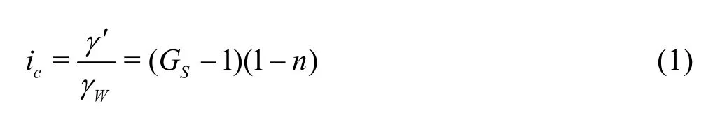
where g¢ is the submerged or effective soil weight, Wg is the water weight,SG is the specific gravity of the soil and n is the porosity of the soil. It is possible to distinguish several stages in fluidisation problems:

(1) The soil grains may remain fixed as long as the fluid drag on each soil grain remains low (static equilibrium).

(2) Increasing the inflow velocity, the upward drag force starts to offset the gravitational forces and the soil expands in volume (heave).

(3) At the critical hydraulic gradient, the drag forces exactly equal the gravitational forces and the bed will begin to behave like a fluid. At this stage the soil grains are in suspension but their net vertical displacement is equal to zero (incipient fluidisation stage).

(4) The bulk density of the soil will decrease if the hydraulic gradient is further increased. Segregation will occur and the fluidisation can be classified as particulate or aggregative in behavior. The particulate behavior occurs when the expansion of the bulk is roughly uniform. The aggregative behavior is characterized by more violent local expansions including air bubbles and fluid pockets.

The incipient fluidisation stage is reached when the following two conditions occur at the same time: the ective stress reaches zero and the specimen expands sufficiently such that the solid matrix, the ensemble of soil grains, loses its structure[1]. Assuming a particulate behavior the expansion of the bulk can be depicted using the soil porosity value. It is also possible to define the maximum porosity as an intrinsic property of the soil. This value will depend on grain size distribution, friction angle, shape factor, segregation, preparation technique and other factors.

Experiments by Vardoulakis[4]show that by increasing the flow rate stepwise above the critical value for incipient fluidisation (Eq.(1)), it is possible to observe a porosity expansion wave that propagates upwards at a constant velocity with a constant linear front as shown in Figs.1(a), 1(b). Nevertheless, on a longer time scale, non-linear effects become significant and must be included. Increasing the flow rate up to and above the critical hydraulic gradient causes the sand to expand. The laboratory experiments confirmed that, after the incipient fluidisation state, increasing the flow rate causes a new equilibrium state to occur for hydraulic gradients i > icr. The experimental results also support a non-linear relation between the fluid flow rate and the hydraulic gradient.

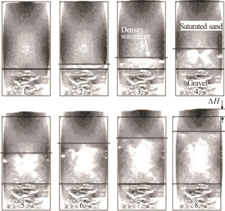
Fig.1(a) X-ray tomography images from fluidized column experiments, illustration of an upwards propagating rarefaction density wave[2]

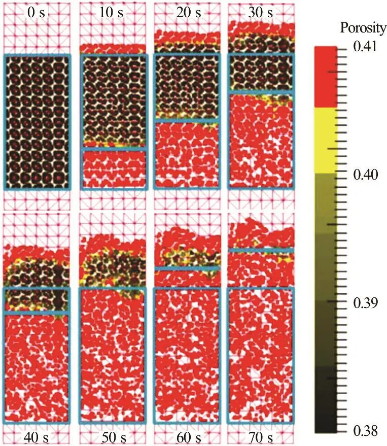
Fig.1(b) (Color online) Density wave propagation visible in MPM fluidisation simulations with initial hydraulic gradient i =1.5, the MPs representing the sand turns red when the porosity exceeds the maximum value nm ax(fluid state)

Concerning the behavior of the bed prior to fluidisation, the best fit between the hydraulic resistivity and the flow rate is depicted by Darcy-Forchheimer law[4].

2. Physical modelling

In order to compare the results of MPM simulations with experimental data, a vertical column testhas been set-up at Deltares, Delft, The Netherlands. Three tests have been performed which yielded similar results.

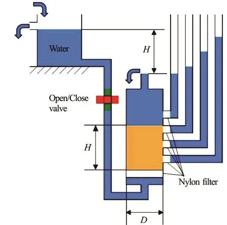
Fig.2(a) (Color online) Sketch

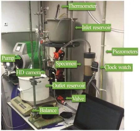
Fig.2(b) (Color online) Laboratory set-up used for fluidisation physical modelling

The specimen is built in a transparent cylinder (Fig.2). The averaged internal diameter D and the effective internal height H of the cylinder are respectively 79.8 mm and 186 mm. A valve allows the connection with an upstream water reservoir with known hydraulic head. The water flows through a U-shaped tube, then into an empty chamber with a plastic frame closed by a low resistance nylon filter. This set-up it is required to:

(1) Provide a regular permeable floor to the soil specimen.

(2) Avoid back-flow of sand.

(3) Provide a uniform velocity field of the water inflow from the base.

(4) Minimize the flow resistance interference.

The permeability of the nylon filter is estimated to be at least 50 times the expected permeability of the soil. The soil sample is built on top of the filter. The sand specimen has a uniform grain size distribution to reduce the effect of segregation during the preparation and in post fluidisation conditions. The sand specimen is prepared in submerged conditions. Preparation of the specimen is performed by casting shallow layers by wet pluviation. The porosity and the sand density are estimated considering the density of the sand grains, the poured sand weight and its volume inside the cylinder of known dimensions. Compaction was performed by means of vertical shock-waves as described by Van der Poel[5]. The minimum and maximum porosity n of the sand are respectively 0.3201 and 0.4106 in dry conditions. For the preparation of the sand specimen a low relative density of 40% was chosen to achieve a highly susceptible soil for fluidisation. It is then possible to assume that the porosity of the bulk will be equal to 0.38 if homogeneously distributed.

The cylinder is finally filled to the top with deairated water. According Van der Poel[5]the error on expected porosity is in the order of 0.9% with the only exception of a shallow top layer with lower porosity. At the outflow, a reservoir of known weight on a balance with an accuracy of 50 g± m , allows the manual measurement of the water flow every 10 s. The whole experiment is registered with a camera and real time clocks. Hydraulic head and specimen expansion are recorded by means of graduated meters with an accuracy of 0.5mm± . Every 5 s a high definition camera took a picture of the specimen to access the deformation of the specimen.

Table 1 Input parameters for MPM simulation with initial hydraulic gradient=1.5i

The parameters of the sand were determined by standard laboratory testing and are collected in Table 1.

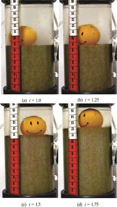
Fig.3 (Color online) Visual inspection of soil behaviour in physical model tests

In this section the behavior of the soil during the test is described based on the test results as shown in Figs.3(a)-3(d). The soil specimen during visual inspection does not show effects of liquefaction for hydraulic gradients up to 1.25 (Figs.3(a), 3(b)) (the critical hydraulic gradient for liquefaction was 1.03 for the test in analysis): the bulk slightly expands but the sand grains do not experience visually detectable displacements. However, whenever the surface is deformed by an external body, it returns to a flat configuration which means that, at least at the surface, the sand is in liquid state already. Moreover, at this stage it was not possible to observe segregation of the sand grains along the specimen. Further increasing the hydraulic gradient up to 1.5 (Fig.3(c)) major segregation processes started with some piping phenomena (aggregative behavior), therefore the hydro-dynamically stable media assumption drops. Once a pipe was observed, the channel was stable only for a few seconds and migrated along the wall of the cylinder in an unpredictable motion. Close to the main stream channel some vorticity of the sand grains was visible. At very high hydraulic gradients, the sand grains were subjected to a very chaotic motion similar to boiling water. The layering effect of segregation was now clearly visible, also at a long distance from the specimen. Further results are discussed in the following “Comparison of results” section.

3. Numerical modelling

The MPM is an arbitrary Lagrangian-Eulerian technique that uses a MP discretisation together with a standard finite element computational grid for the representation of time dependent continuum bodies. The MPs represent the considered body and they carry all the physical properties as well as external loads while the finite elements and their Gauss points carry no permanent information but are used only for computational purposes. At the beginning of the time step the physical properties are mapped from the MPs to the nodes of the mesh. The MPs must represent volumes sufficiently small to treat the properties average values like local variables and sufficiently big to make the fluctuations of these values negligible over the volumes. The incremental solution of the basic equations is computed according to classic Lagrangian FEM computation. At the end of the time step the solution is mapped back from the mesh in order to update the MPs information.

The computational mesh is then reset to its initial configuration[6]. The recently developed double point formulation[1]allows assigning to each phase (the solid and the liquid one) a set of MPs and simulate their coupled behavior by means of the interaction force. The motions of both MP sets are described by a system of momentum balance equations using separate velocity fields for the solid and the liquid constituent. When the grains of the solid constituent are in contact and the behavior of the soil can be described by continuum constitutive models for granular materials, the sample is defined to be in solid state. As soon as the effective stress in the MP is becoming nil and the porosity exceeds its maximum value the solid constituent will be described by Navier-Stokes equations and it is defined to be in liquid state.

Using the double point MPM formulation the vertical column tests are modelled numerically. The model schematisation, dimensions and mesh discretisation are shown in Figs.4(a), 4(b). The upstream reservoir has sufficient dimensions to approximate a constant hydraulic head.

The dimensions of the model are chosen such that it was possible: to vary the hydraulic gradient around its critical value for fluidization of the sand specimen and, to allow the bulk expansion of the sand specimen. Tetrahedral structured uniform mesh elements are used which have linear shape functions. Stresses are initialised by a gravity loading phase for which numericaldamping is applied to converge with quasi-static equilibrium state. Perfectly smooth contact with the walls of the model is assumed for both of the constituents. Opening a water-permeable gate boundary condition at the bottom of the sand column allows to apply the designed hydraulic gradient. The input parameters are shown in Table 1.

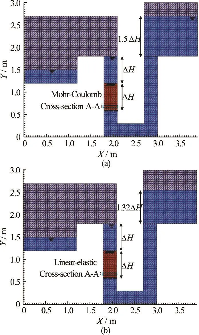
Fig.4 (Color online) Model schematisation and mesh used for fluidisation numerical analysis with: (a) Mohr-Coulomb constitutive model and initial hydraulic gradient i0=1.5 . (b) Linear elastic constitutive model and reduced hydraulic head upstream to simulate the expanded bulk in steady state conditions

4. Comparison of results

4.1 MPM vs. analytical

The flow velocity field of the liquid MPs was an average of all the MPs present at time =0st in the region highlighted in Figs.4(a), 4(b) representing a generic horizontal cross-section A-A in the specimen. Assuming steady state conditions, Forchheimer’s equation provides an analytic estimation of the fluid flow velocity. This formula is used to take in account the high velocity inertia effects adding a second order term in Darcy’s law

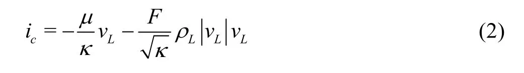
where i is the hydraulic gradient, m dynamic viscosity, k intrinsic permeability,Lv Darcy’s velocity, F Ergun’s coefficient andLr density of the water. The Ergun’s coefficient F is computed as

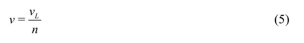
where A and B are the Ergun’s Law constants[7]. The same Kozeny-Carman formula[8]implemented in the code was therefore here applied to estimate the intrinsic permeability value

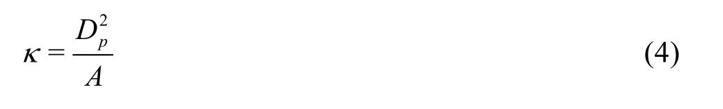
wherepD is the equivalent grain size diameter and n is the bulk porosity. The fluid velocity v is related to the Darcy’s velocityLv by the porosity n. The Darcy’s velocity is divided by porosity to account for the fact that only a fraction of the total formation volume is available for flow. The fluid velocity would be the velocity a conservative tracer would experience if carried by the fluid through the formation.

The velocity field calculated from MPM simulation can not be directly compared to the analytic solution. The constant Ergun’s coefficient F is valid as long as the fluid flow is laminar. Thus, in high velocity flow regime, Ergun’s coefficient F needs to be adapted to reflect the experimental inertial effects that are currently neglected. To overcome this limit, two simulations are performed (Figs.4(a), 4(b)): simulation A (Fig.4(a)) for the bulk expansion with Mohr-Coulomb constitutive model, simulation B (Fig.4(b)) for the flow velocity field analysis with linear elastic constitutive model.

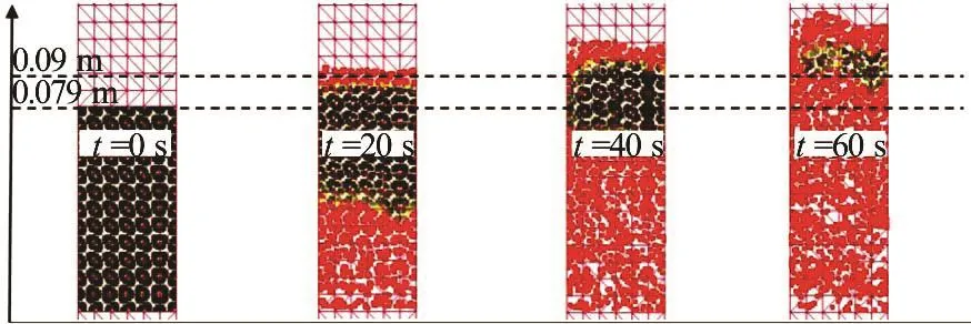
Fig.5(a) (Color online) Bulk expansion images from MPM simulation

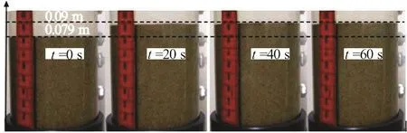
Fig.5(b) (Color online) Vertical sand column test expansion with initial hydraulic gradient equal to =1.5i

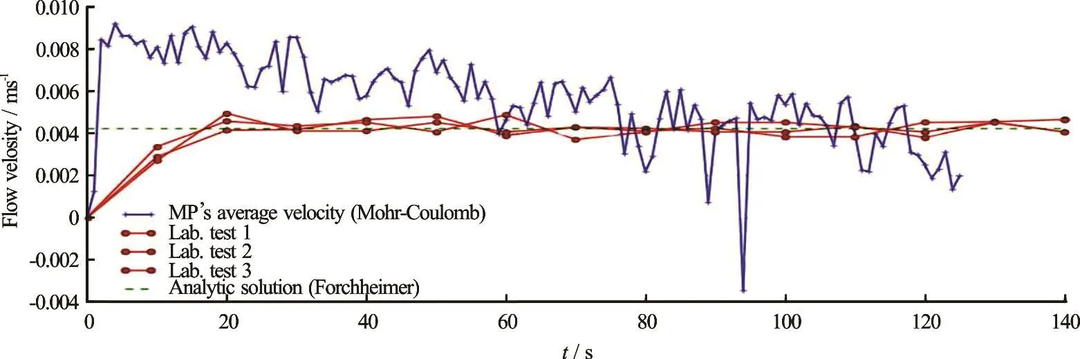
Fig.5(c) (Color online) Filter velocity plot of MPM simulation compared with analytical and physical model results

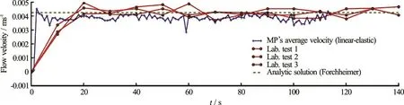
Fig.6 (Color online) Filter velocity plot of MPM simulation compared with analytical and physical model results

The simulated expansion of the bulk and flow velocity are considerably higher than those measured in the laboratory experiment (Figs.5(a)-5(c)). The final bulk expansion was recorded in laboratory, after steady regime conditions were achieved. These values can now be used to design a new numerical model by reducing the hydraulic gradient to reflect the experimental results: the new geometry (Fig.4(b)) depicts the applied hydraulic gradient, porosity and fluid path length measured in laboratory. In the simulation with Mohr-Coulomb constitutive model, the higher bulk expansion may be caused by the continuum approach that, at the moment, does not include the influence of localized phenomena (inertia effects, piping, faults, internal erosion and segregation) that in experimental results dissipates part of the flow energy.

The second simulation was therefore run with linear-elastic constitutive model. The porosity and specimen size can now be considered constant during the whole simulation. Final porosity, bulk length and hydraulic gradient at steady regime conditions assume respectively the values n =0.452, H =90mm and i =1.32 consistently to the measurements performed during laboratory experiments. Furthermore, since the MPs representing the water have same mass and same volume, it was possible to average arithmetically their superficial fluid flow velocity. In Fig.6 the averaged flow velocity time evolution for simulation B is shown. The blue line is the time evolution of the water flow velocity derived from MPs present in section A-A at time equal to zero and it is compared with the analytic result given by the Darcy-Forchheimer law plotted in dashed green line. In red the averaged velocities measured during laboratory experiments are also reported every 10 s. The (initial) transient part of the physical models takes place probably due to the bulk expansion. No bulk expansion takes place when the linear elastic constitutive model is applied. Nevertheless, if we neglect this initial transient phase and we take in analysis only the averaged flow velocity in steady regime condition, the simulation results show good agreement with the analytical solution (Eq.(2)).

4.2 Physical vs. analytical

The laboratory test results are compared, with the analytical expression of the filter velocity (Eq.(2)). For the three tests with initial hydraulic gradient =1.5i the sand grains were moving due to some piping and segregation motion so it is possible to assume that the specimen was liquefied.

The correspondent analytic solution must take in account the expansion and porosity values of the bulk in steady state conditions. Some oscillation of data in the physical model around the analytic filter velocity value may be due to the manual measurement of the outflow. The bulk porosity was derived by visual inspection of the sand specimen expansion. To evaluate the correspondent analytical velocity values, the steady regime conditions pressure gradient, bulk density and the length of the sand specimen are taken into account. The two solutions are considered matching with high accuracy.

4.3 MPM vs. physical

The input parameters for the MPM simulation are defined to describe as close as possible the vertical column test previously introduced in Section 3. The flow velocity calculated with MPM also matches with high accuracy those measured with the three vertical column tests. However, the MPM simulation A (Fig.4(a)), even representing qualitatively the bulk expansion, does not show final values as expected from the physical test (Fig.5(c)). In fact, the expansion of the specimen occurs slower than in the laboratory experiment. In Figs.5(a)-5(c) it is possible to see the expansion in MPM with Mohr-Coulomb constitutive model versus the laboratory experiment measurements.

The descending trend of the MPM water velocity is considered mainly due to the decreasing water head in the up hill reservoir.

5. Conclusion

The analysis of the simulations of vertical column tests showed that the advanced MPM double point formulation is able to catch the qualitative and quantitative behaviour of a sand specimen subjected to fluidisation. In the performed numerical simulations different aspects related to fluidisation were observed, including the general linear expansion wave front at a constant velocity as explained by Vardoulakis[4](Fig.1). Also the quantitative estimation of seepage flow can be performed after calibration derived from physical modelling for the case study in analysis. The presented double point MPM formulation can therefore be applied to model large deformation problems in geo-mechanics that involve coupling of soil deformations with pore water pressure and fluid flow induced by a hydraulic gradient[9].

[1] Martinelli M. Layer formulation: Joint MPM Software [M]. Deltares, Delft, The Netherlands: MPM Research Community, 2015.

[2] Vardoulakis I., Stavropoulou M., Skjaerstein A. Porosity waves in fluidised sand-column tests [J]. Transactions Royal Society London Ser. A, 1998, 356: 25912608.

[3] Terzaghi K. Erdbaumechanik auf bodenphysikalischer grundlage [M]. Wien, Austria: Deuticke, 1925.

[4] Vardoulakis I. Fluidisation in artesian flow conditions: Hydro-mechanically stable granular media [J]. Geotechnique, 2004, 54(2): 117-130.

[5] Van der Poel J. T., Schenkeveld F. M. A preparation technique for very homogenous sand models and CPT research [C]. Centrifuge 98: Proceedings of the International Conference Centrifuge 98. Tokyo, Japan, 1998.

[6] Stomakhin A., Schroeder C., Chai L. et al. A material point method for snow simulation [J]. ACM Transactions on Graphics, 2013, 32(4): 102-113.

[7] Ergun S., Orning A. A. Fluid flow through packed columns [J]. Chemical Engineering Progress, 1952, 48: 89-94.

[8] Bear J. Dynamics of fluids in porous media [M]. New York, USA: Elsevier, 1972.

[9] Bandara S., Soga K. Coupling of soil deformation and pore fluid flow using material point method [J]. Computers and Geotechnics, 2015, 63: 199-214.

[10] Anura3D MPM Research Community: www.anura3d.com [EB/OL].

Acknowledgements

I want to thank Alex Rohe for his precious supervision, contributions and friendship. For the numerical simulations the Anura3D software of the MPM Research Community[10]is used, which is greatly acknowledged. This work was performed as a partial contribution to obtain a MSc degree at Bologna University, Italy. The work was performed at Deltares, in collaboration with the Delft University of Technology Chair of Hydraulic Structures.

10.1016/S1001-6058(16)60753-9

February 17, 2017, Revised March 15, 2017)

*Biography:Marco Bolognin, Male, Ph. D. Candidate