Poroelastic solid flow with double point material point method*

Bruno Zuada Coelho, Alexander Rohe, Kenichi Soga

1. Department of geo-engineering, Deltares, Delft, the Netherlands, E-mail: Bruno.ZuadaCoelho@deltares.nl

2. Department of Engineering, University of Cambridge, Cambridge, UK

Poroelastic solid flow with double point material point method*

Bruno Zuada Coelho1, Alexander Rohe1, Kenichi Soga2

1. Department of geo-engineering, Deltares, Delft, the Netherlands, E-mail: Bruno.ZuadaCoelho@deltares.nl

2. Department of Engineering, University of Cambridge, Cambridge, UK

2017,29(3):423-430

This paper presents the numerical modelling of one and two-dimensional poroelastic solid flows, using the material point method with double point formulation. The double point formulation offers the convenience of allowing for transitions in the flow conditions of the liquid, between free surface flow and groundwater flow. The numerical model is validated by comparing the solid flow velocity with the analytical solution. The influence of the Youngʼs modulus on the solid flow velocity is discussed for both one and two-dimensional analysis cases. The effect of the shape of the two-dimensional solid is investigated. It is shown that the solid stiffness has an effect on the poroelastic flow velocity, due to swelling and bending for the one and two-dimensional cases, respectively. The shape is found to be an important factor on the flow velocity of the poroelastic solid.

Material point method, geocontainers, double point formulation, large deformations

Introduction

The modelling of large deformations is of great importance for engineering problems. The material point method (MPM) is a mesh-free method that has beendeveloped to address the problem of large deformation on a continuum level. The continuum material is represented by a set of Lagrangian points (material points) that move through an Eulerian background mesh. The material points contain all the properties of the continuum, such as mass, stress, strain and material parameters. Therefore, MPM can be seen as a combination of both Lagrangian and Eulerian formulations. The problems related to mesh distortion under large deformations are circumvented, as well as the diffusion associated with the convective terms of the Eulerian approach[1,2]. The use of Lagrangianmaterial points conserves mass and allows history-dependent material models to be used. The discrete equations for the momentum balance equations are obtained on the background grid similar to the finite element method with an updated Lagrangian formulation.

MPM has been used with success for geomechanics problems using the single point formulation[3-5], where both the solid and liquid are described by thesame Lagrangian material point. However, this formulation is not appropriate to simulate problems involving the interaction between solid and liquid, as often is the case for offshore applications. To overcome this limitation, a double point formulation has previously been developed[6,7]. This formulation extends the classical two-phase approach to model saturated solids[8], which cannot capture the transition in state for both liquid and solid phases. The key aspect of this new formulation is that it considers two sets of Lagrangian material points to represent solidand liquid. The motion of both sets of material points is described by means of the momentum balance equations, using separate field velocities for both the solid and liquid phases. This means that each of the two constituents can move in respect to each other and both interact by means of a drag force.

Using the double point formulation, problems involving the fluidisation and sedimentation of solidliquid mixtures can be modelled, as well as problems where free surface liquid flows through a porous solid (i.e., a transition ofthe liquid state from free surface flow to groundwater).

Geocontainers are sand filled bags encapsulated by a geotextile membrane, often used for coastal applications, such as revetments and breakwaters, mainly due to its resistance to erosion. The modelling of geocontainers is one of the many offshore applicationsthat illustrates the necessity of the double point formulation. Although the single point formulation is not the most appropriate strategy to model the installation of geocontainers, it has been the most widely used methodology[9-12]. The need for the double point formulation is related to the requirementto model both large deformations, and the interaction between the solid and liquid materials, and the change in flow conditions of the liquid (between free surface and groundwater flow), as the liquid flows around and through the solid.

In the present paper, two problems where the transition of the liquid conditions occurs are analysed: one- and two-dimensional poroelastic flow through a porous solid immersed inside a Newtonian liquid. The latter resembles a geocontainer. The influence of the Youngʼs modulus on the flow velocity of the falling solid by gravity, and the deformation of the modelled geocontainer will be discussed.

1. One-dimensional poroelastic solid flow

1.1 Analysis description

The numerical analyses of poroelastic solid flow have been performed with the MPM software Anura3D[13], following thedouble point formulation to simulate the interaction between solid and liquid[7]. The validation of the MPM implementation has been performed by simulating an one-dimensional poroelastic solid falling through a Newtonian liquid by gravity. This problem was chosen as it offers the convenience of having a closed form analytical solution for the steady state velocity of the poroelastic solid flow.

Fig.1 Geometry of the poroelastic solid and water column

The geometry of the problem is shown in Fig.1. The dimensions H and L were assumed as 0.1 m and 1 m, respectively. The system of equations is solved explicitly in the time domain. The domain was discretised using low-order tetrahedral elements (in total 780 elements), with initially ten solid and ten liquid material points for the elements filled with saturated poroelastic solid and ten liquid material points for the elements filled with liquid only. The nodes at the bottom of the column were fixed in the vertical direction.

The solid material is assumed to be linear elastic and the liquid material is modelled as compressible Newtonian liquid. Table 1 presents the material properties.

Table 1 Material properties for the poroelastic solid flow

1.2 Analytical solution

The steady state velocity of a rigid poroelastic solid falling through a liquid by gravity offers the convenience of an analytical solution[14]. The velocity v of the solid follows

where g¢ represents the submerged volumetric weight,k the intrinsic permeability, and F the coefficient from Ergunʼs drag force[15]

with parameters A and B being, respectively, 150 and 1.75[15]. The intrinsic permeability k is defined as[16]

where Dsis the grain size diameter.

1.3 Results

1.3.1 Validation of the numerical results

Figure 2 ashows the comparison between the analytical and numerical results for the one-dimensional poroelastic solid flow. Results show that the numerical results obtained with MPM are in agreement with the analytical solution. Due to the high permeability (solid grain diameter Ds) the transient behaviour of the flow is not noticeable in Fig.2.

Fig.2 (Color online) Comparison between the analytical and numerical results

The velocity computed with MPM oscillates around the analytical value (Fig.2(b)), initially (up to normalised time 0.1) with a sinusoidal shape, followed by a non-periodic oscillationsat greater times. The sinusoidal oscillation is related to the fact that the liquid is modelled as a compressive material, and will be discussed in the next section. The non-periodic oscillation is caused by element crossing, due to the discontinuity in the liquid concentration ratio, at the boundary between the liquid and the solid.

1.3.2 Liquid bulk modulus

The poroelastic solid velocity was found to have a sinusoidaloscillation around the analytical value. In order to gain insight into the causes of this oscillation, Fig.3 presents the flow velocity for different values of the bulk modulus of the liquid (Kl). Results show that the sinusoidal oscillation is related to the liquid compressibility. As liquid compressibility increases, the frequency of the oscillation increases, and the amplitude decreases. At the bottom of the column the movement of the liquid material points is restrained, due to the fixed boundary conditions. As the liquid has a compressibility Kl, the poroelastic solid oscillates on the top of the liquid due to its inertial force. This system can be idealised as a mass spring system, where the poroelastic solid represents the mass, and the spring corresponds to the liquid. The natural frequency w of the mass spring system is defined as

where k and m are, respectively, the spring stiffness and solid mass. The free vibration solution of a mass spring system follows

As the spring stiffness k increases (in this case the liquid bulk modulus), the amplitude of the oscillation decreases and its frequency increases (consistent with the results in Fig.3).

Fig.3 (Color online) Effect of the liquid bulk modulus on the poroelastic flow velocity

This is further illustrated in Fig.4, which shows the effect of the liquid column length H on the amplitude and frequency of the vibration. It is clear that as the length of the liquid column is increased by a factor of 2 and 4, the main frequency of oscillation is reduced by a factor ofrespectively, consistent with Eq.(4). When the length of liquid column increases by a factor i, it corresponds to a reduction of the stiffness by the same factor i (Fig.4). The sinusoidal oscillation related to the liquid compressibility can be solved by adopting an incompressibleformulation for the liquid[17,18].

Fig.4 (Color online) Effect of the liquid column length on the velocity oscillation

1.3.3 Solid Young modulus

The effect of solid Young’s modulus on the onedimensional poroelastic flow problem was investigated for a range of values between 50 kPa and 50 MPa. The grain size diameter was 5´10-4m, to which corresponds an intrinsic permeability of =k 2.96×10‒10m2(Darcy permeability: K =2.96´ 10-3m/s ). The grain sizediameter (porosity) was reduced in relation to the previous analysis, in order to capture the transient behaviour of the poroelastic solid.

Figure 5(a) presents the results for several Young’s modulus cases. The transient behaviour of the poroelastic solid can beclearly identified for the casewith a Young modulus of 50 kPa. Up to a normalised time of 0.004 the solid is accelerating, after which it reaches the steady state velocity. This transient behaviour is related to the swellingthat develops during the flow. The flow occurs because there is a pressure gradient between the top and bottom of the solid, which causes an excess pore water pressure at the bottom. This results in the occurrence of dissipation of the excess pore water pressure and swelling of the poroelastic solid (i.e., extension).

For the remaining cases of higher Youngʼs modulus, the transient response is less noticeable. This is caused by a faster swellingand a smaller extension of the solid. This is illustrated in Fig.5(b), which shows the solid extension for the different Young’s modulus cases. It is clear that the smaller the Youngʼs modulus is, the larger the solid extension is. For the cases of Youngʼs modulusof 5 000 kPa and 50 000 kPa, the extension is negligible.

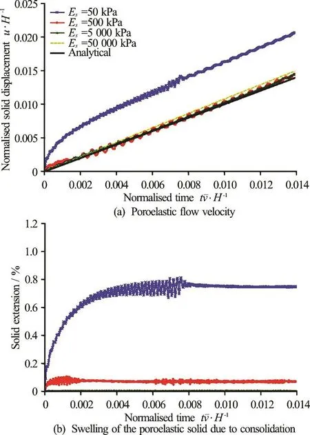
Fig.5 (Color online) Effect of the solid Young’s modulus

Fig.6 (Color online) Normalised extension of the poroelastic solid due to consolidation (bold line represents moving average)

The extension of the poroelastic solid can be expressed as a function of the consolidation time T, defined as

where cvcorresponds to the consolidation coefficient and d is the drainage path length. Figure 6 showsthat the numerical results for the normalised extension of the poroelastic solid (defined as the ratio between the extension and the maximum extension) follow the trend of the analytical solution for the one-dimensional consolidation problem (oedometer consolidation)[19]. The differences between the two results are related to the fact that the poroelastic flow does not have the same boundary conditions as the oedometer test, as the solid is moving, combined with liquid pressure fluctuations at the interface between the solid and liquid materials due to numerical issues.

The solid velocity oscillates significantly around the average value for the softer solids ( E=50kPa and E=500kPa ). These oscillations are likely related to the fact that these solids experience more extension, hence more liquid pressure oscillations within the solid.

2. Submerged two-dimensional poroelastic solid flow

2.1 Analysis description

This section presents the modelling results of a two dimensional poroelastic solid flow case, which resembles a simplified geocontainer installation process, and shows the appropriateness of the MPM double point formulation for the analysis of this type of problem.

Fig.7 Geometry of the two-dimensional poroelastic flow (simplified geocontainer)

Figure 7 shows the geometry of the problem (dimensions assumed as: H =1m, L =2m and B =4m ). The problem is assumed to be symmetric, with the nodes at the bottom of the model fixed in the vertical direction, and at the side in the horizontal direction. In total the model comprised 6 300 elements with the following material point distribution:

(1) 10 materials points for solid and liquid phase respectively in the poroelastic material.

(2) 20 materials points for the liquid phase in the liquid material.

Table 2 Material properties for the two-dimensional poroelastic solid flow

Fig.8 (Color online) Flow of the two-dimensional poroelastic solid at times

The solid material is assumed to be linear elastic and the liquid material is modelled as compressible Newtonian liquid. Table 2 presents the adopted properties for the solid and liquid materials.

2.2 Overall response

Figure 8 shows, at several distinct times, the movement of the poroelastic solid through the liquid. For the chosen parameters (i.e., stiff and low permeability geocontainer), the poroelastic solid is found to move down through the liquid as a rigid body, i.e., without significant bending.

From the figure it is possible to see that the liquidflows into the bottom of the solid.The blue material points (initially liquid material points) enter the domain of the black material points (solid material points). The green material points (initially groundwater liquid material points) flow out of the top of the solid and leave the domain of the black material points (solid material points). However, in this case, the movement of the solid is mainly due to the liquid that flows around the solid, rather than through it.

2.3 Solid Young modulus

The effect of solid Youngʼs modulus on the twodimensional poroelastic flow problem was investigated for three different values: 500 kPa, 5 000 kPa and 50 000 kPa. All remaining properties were the same as presented in Table 2.

Fig.9 (Color online) Effect of the solid Young modulus

Figure 9 shows the effect of Youngʼs modulus on the solid vertical displacement and the velocity for Point A (see Fig.7). The velocity is found to increase with the reduction of the solid Young modulus. This increase insolid velocity is related to the bending deformation of the poroelastic solid. As the stiffness decreases, the solid exhibits higher deformation due to bending as the water flows around the solid. As the solid bends, the water flow around it is facilitated, and the solid velocity increases. This is illustrated in Fig.10, which shows the poroelastic solid displacement for a Young modulus of 500 kPa at =5st (Fig.8(d) shows the poroelastic solid displacement at the same time).

Fig.10 (Color online) Deformation of the poroelastic solid for a Young modulus of 500 kPa at =5st

2.4 Solidgeometry

The effect of the solid geometry was evaluated by comparing three different widthsof the poroelastic solid ( =1mB , =2mB and =4mB -see Fig.7). The distance L was kept the same for all analyses, and was equal to 1 m. Figure 11 shows that, as the width is reduced, the falling velocity increases. This is related to the fact that, as the block is smaller, the flow of the liquid around the block is facilitated. However, the relation between the solid width and flow velocity is not linear. This means that, when the block width is reduced by a factor of 2, the falling velocity doesnot increase by the same factor.

The effect of the poroelastic solid height was studied for three different values ( H =0.25m , H= 0.5 m and H =1m-see Fig.7), assuming a constant width B =4m. Figure 12 presents the comparison of the falling flow displacement and the velocity for the different height cases. As the height of the poroelastic solid increases, the faster it falls. This is because asthe height of the poroelastic solid increases, so does its weight. This further illustrates that the poroelastic flow is governed by the flow around the solid, and not through it, in this particular cases. The cases with higher permeability will be performed as future study in order to examine the effect of liquid flowing through the solid on the solid behaviour.

Fig.11 (Color online) Effect of the solid width

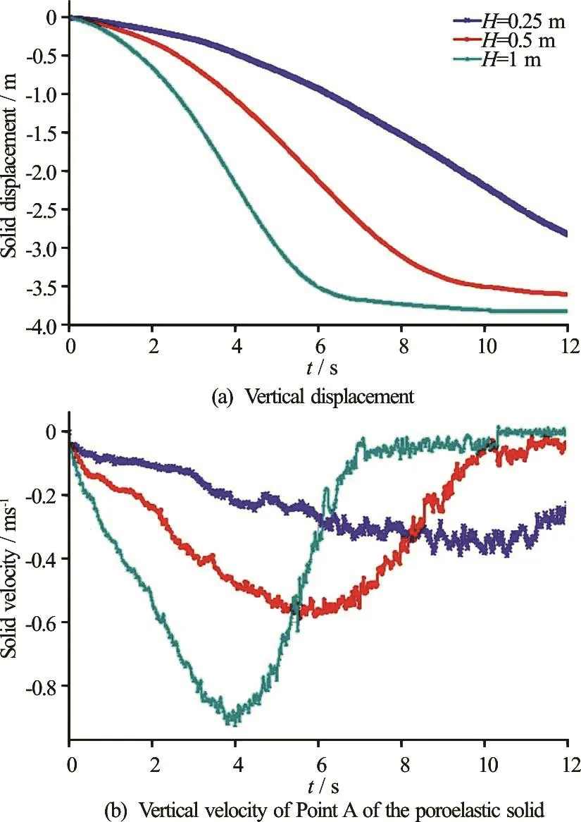
Fig.12 (Color online) Effect of the solid height

3. Conclusions

This paper presented the validation and two numerical applications of the MPM double point formulation[6,7].

The one-dimensional poroelastic flow was used to illustrate the accuracy of the numerical results. Additionally, it was shown that there is a transient response of the poroelastic flow velocity, where the solid swells due to solid. The poroelastic solid velocity was found to have a sinusoidal oscillation around the analytical flow velocity, due to the liquid compressibility, and element crossing. However the average value of the velocity is inagreement with the analytical solution. A possible mitigation for these oscillations can be the implementation of incompressible liquid, and a redefinition of the transition zone between solid and liquid to address the discontinuity in the liquid concentration ratio. Further study is required to solve this issue.

The two-dimensional poroelastic analysis resembled the installation of a geocontainer. It was found that the flow velocity of the falling poroelastic solid depends on the solid Young’s modulus, and on its shape for a given permeability value used for the simulations. As the solid Young modulus reduces, the solid bending curvature is greater, which improves the flow around the solid, therefore the solid velocity is higher. The flow velocity was found to increase for narrow and thicker poroelastic solids. As the velocity of the falling poroelastic is governed through the flow of liquid around the solid, narrow solids fall faster. By increasing the height of the solid, its weight will increase which will also increase the falling velocity of the poroelastic solid. Further work is needed to examine the effect of permeability on the solid behaviour.

Acknowledgements

[1] Sulsky D., Schreyer H. Particle-in-cell method as a naturalimpact algorithm [J]. Advanced Computational Methods for Material Modeling, 1993, 268: 219-229.

[2] Sulsky D., Chen Z., Schreyer H. A particle method for history-dependent materials [J]. Computer Methods in Applied Mechanics and Engineering, 1994, 118(1-2): 179-196.

[3] Więckowski Z. The material point method in large strain engineering problems [J]. Computer Methods in Applied Mechanics and Engineering, 2004, 193(39-41): 4417-4438.

[4] Coetzee C., Vermeer P., Basson A. The modelling of anchors using the material point method [J]. International Journal for Numerical and Analytical Methods in Geomechanics, 2005, 29(9): 879-895.

[5] Alonso E. E., Zabala F. Progressive failure of Aznalcóllar dam using the material point method [J]. Géotechnique, 2011, 61(9): 795-808.

[6] Bandara S., Soga K. Coupling of soil deformation and pore fluid flow using material point method [J]. Computers and Geotechnics, 2015, 63(1): 199-214.

[7] Martinelli M., Rohe A. Modelling fluidisation and sedimentation using material point method [C]. 1st Pan-American Congress on Computational Mechanics. Buenos Aires, 2015.

[8] Zienkiewicz O., Chan A., Pastor M. et al. Computational geomechanics [M]. New York, USA: John Wiley and Sons, 1999.

[9] Więckowski Z. Enhancement of the material point method for fluid-structure interaction and erosion [R]. Seventh Framework Programme, 2013.

[10] Grabe J., Heins E., Qiu G. et al. Numerical investigation of loading on geotextile sand containers [C]. 10th International Conference on Geosynthetics. Berlin, Germany, 2014.

[11] Hamad F., Stolle D., Vermeer P. Modelling of membranes in the material point method with applications [J]. International Journal for Numerical and Analytical Methods in Geomechanics, 2015, 39(8): 833-853.

[12] Hamad F., Więckowski Z., Moormann C. Interaction of fluid–solid–geomembrane by the material point method [J]. Computers and Geotechnics, 2017, 81: 112-124.

[13] Anura3D. www.anura3D.com, Anura3D MPM Research Community [EB/OL].

[14] Martinelli M. Two layer formulation. Joint MPM Software [M]. Delft, The Netherlands: Deltares, 2015.

[15] Ergun S. Fluid flow through packed column [J]. Chemical Engineering Progress, 1952, 48(2): 89-94.

[16] Bear J. Dynamics of fluids in porous media [M]. New York, USA: Elsevier, 1972.

[17] Harlow F., Welch J. Numerical calculation of trime-dependent viscous incompressible flow of fluid with free surface [J]. Physics of Fluids, 1965, 8(12): 2812-2819.

[18] Chorin A. Numerical solution of the Navier-Stokes equations [J]. Mathematics of Computation, 1968, 22(104): 745-762.

[19] Verruijt A. Soil mechanics [R]. Delft, The Netherlands: Delft University of Technology, 2006.

10.1016/S1001-6058(16)60752-7

arch leading to these results has

funding from the European Union Seventh Framework Programme (FP7/2007-2013) under grant agreement No. PIAP-GA-2012-324522 “MPM-DREDGE”. This paper has been partially published in the Proceedings of the 1st International Conference on the Material Point Method (MPM 2017), 10-13 January 2017, Delft, The Netherlands,

10.1016/j.proeng.2017.01.035.

(Received February 15, 2017, Revised March 22, 2017)

*Biography:Bruno Zuada Coelho, Male, Ph. D., Engineer