Local and biglobal linear stability analysisof parallel shear flows

Sanjay Mittal and Anubhav Dwivedi

1 Introduction

Thehydrodynamic stability of laminar flows has received significant attention and has been investigated by several researchers in the past[Schmid and Henningson(2001);Chandrasekhar(1981);Huerre and Monkewitz(1990);Huerre(2000);Chomaz(2005)].The linear stability of parallel shear flows can be analyzed via finding solution to the Orr-Sommerfeld (OS) equation [Orr (1907); Sommerfeld(1908)], with suitable boundary conditions. The disturbance fi eld is assumed to be a plane wave whose amplitude varies transverse to the flow and is periodic in the homogeneous directions. The analysis can be carried out in either a spatial or temporal framework [Boiko, Dovgal, Grek, and Kozlov (2012)]. The spatial analysis assumes that the disturbance field develops in s pace. The spatial growth rate is determined for different values of frequency and Reynolds number. In contrast, the temporal analysis assumes that the disturbance develops in time. As per the Squire’s theorem [Schmid and Henningson (2001)], the 2D disturbance is the most critical in terms of its growth rate. Therefore, it is suffi cient to consider twodimensional disturbances that have streamwise periodicity [Boiko, Dovgal, Grek,and Kozlov (2012)]. The analysis is carried out to determine temporal growth rate at various Re and for disturbances with different values of streamwise wavenumber. The spatial and temporal approaches for local analysis are related to each other[Huerre (2000)]. For example, Gaster (1962) proposed a transformation for that,approximately, relates the temporal and spatial growth. Several methods have been used to solve the OS equations. Davey and Drazin (1969) utilized Bessel functions to represent the disturbance fi eld and analyze the stability of pipe Poiseuille flow. Orszag (1971) used Chebyshev polynomials to solve the OS equation for the plane Poiseuille flow. Saraph, Vasudeva, and Panikar (1979) used Galerkin’s weighted residual method to carry out the stability analysis of plane Poiseuille flow and magneto-hydrodynamic flows. Garg and Rouleau (1972) used asymptotic analysis to carry out the linear stability analysis in pipe flow. The method has also been applied, in a local sense, to spatially developing flows [Pierrehumbert (1985); Yang and Zebib (1989); Monkewitz (1988); Chomaz, Huerre, and Redekopp (1988)]. In this approach, the flow profi les at different streamwise stations are analyzed by assuming that each profi le corresponds to an independent parallel flow. The local analysis, at each streamwise station of the flow, involves solving the OS equation,with suitable boundary conditions.

Analternateapproach toinvestigatethelinear stability of fluid flowsisthe BiGlobal and TriGlobal stability analysis[Theofilis(2011);Swaminathan,Sahu,Sameen,and Govindrajan(2011)].Unlike in the local analysis,in this approach the disturbance fi eld is represented globally,including in the streamwise direction.The analysis results in global modes which,depending on the sign of the growth rate,may either grow or decay in the entire computational domain with time.The global analysisisusually muchmorecomputationally expensivethan thelocal one.Such an approach has been used to analyze the global linear stability properties of several non-parallel flows[Mittal(2004);Chomaz(2005);Schmid and Henningson(2001)].Swaminathan,Sahu,Sameen,and Govindrajan(2011)carried out a global linear stability analysis of a diverging channel flow using spectral collocation method.Mittal and Kumar(2003)used astabilized finite element method for the global LSA of stationary and rotating cylinder.Later,Verma and Mittal(2011)used asimilar approachfor carryingout global LSA to investigatetheexistenceand stability of secondary wake mode of a two-dimensional flow past a circular cylinder.Morerecently,Navrose,Meena,and Mittal(2015)carried out LSA of spinning cylinder in auniform flow and identifi ed several unstablethree-dimensional modes for variousrotation ratesof thespinning cylinder.

In the present work,Linear Stability Analysis(LSA)of the plane Poiseuille flow is carried out.Local and global analyses are considered.The solutions to the OS equation for local analysis have been obtained in a temporal framework.A spectral collocation method based on Chebyshev polynomials[Schmid and Henningson(2001)]is used to solve the governing Orr-Sommerfeld(OS)equation.The global LSA of theplane Poiseuilleflow iscarried out using astabilized finiteelement formulation.The governing equationsarecast in theprimitivevariables:velocity and pressure.Equal-order finite-element interpolation functions are used for pressure and velocity disturbancefi elds.Four-noded quadrilateral elementswith bilinear interpolation isemployed.Thestreamline-upwind/Petrov-Galerkin(SUPG)[Brooks and Hughes(1982)]and pressure-stabilizing/Petrov-Galerkin(PSPG)stabilization techniques[Tezduyar,Mittal,Ray,and Shih(1992)]are employed to stabilize the computations against spurious numerical oscillations.The fi nite element formulation results in a generalized eigenvalue-vector problem which is solved using the subspace iteration method[Stewart(1975)].For carrying out the global analysis,we assume periodic boundary conditions at the inflow and the outflow for the disturbancefield.Thisallowsadirectcomparisonof theglobal LSA withthe OSequation.A comparison between the local and global analysis of the plane Poiseuille flow at Re=7000 is presented and is utilized to show the connection between the two analyses.

2 Governing Equations

2.1 Linearized Disturbance Equations

Let,Ω⊂Rnsdand(0,T)be the spatial and temporal domains respectively,where nsdis the number of space dimensions,and letΓ denote the boundary ofΩ.The Navier-Stokesequationsgoverning incompressiblefluid flow are given as:

Hereρ,u andσ are the density,velocity and the stress tensor,respectively.The stresstensor isrepresented asσ =−p I+µ((∇u)+(∇u)T),where p andµ arethe pressure and coeffi cient of dynamic viscosity,respectively.The boundary conditionsarespecified as:

Here,ΓgandΓhare the complementary subsetsof the boundaryΓwhere Dirichlet and Neumann boundary conditionsarespecified,respectively.

To understand the evolution of small disturbances,the unsteady solution is expressed asacombination of steady solution and disturbance:

Here,U and P representthesteady statesolution whosestability isto bedetermined while u′and p′aretheperturbation fields.Substituting thedecomposition given by Eq.(3)in Eqs.(1)and subtracting from them,the equations for steady flow one obtains the evolution equations for the disturbance fields.Further,the perturbations,u′and p′,areassumed to besmall and thenon-linear termsaredropped.The linearized perturbation equationsaregiven as:

Here,σ′is the stress tensor for the perturbed solution.Eq.(4)subjected to the initial condition,u′(x,0)=u′0describes the evolution of small disturbances in the domain,Ω.Theboundary conditionson u′arehomogeneousversionsof thoseused for calculating thebaseflow(Eq.(2)).

2.2 Global Linear Stability Analysis

To conduct a global Linear stability analysis we assume the following form of the disturbancefield,u′and p′

Substituting Eqs.(5)in the linearized disturbanceequations(Eqs.(4))we obtain:

Eqs.(6)representsa generalized eigenvalue problem withλas the eigenvalue and(ˆu,ˆp)as the corresponding eigenmode.The boundary conditions for(ˆu,ˆp)are homogeneous version of those used for calculating the base flow(U,P).In general,the eigenvalue λ = λr+iλiis complex.The growth rate is given by the real part,λrof the eigenvalue whereas the imaginary part,λiis related to the temporal frequency of the of the disturbance field.A positive value ofλrindicates an unstable mode.This method has been utilized by several researchers in the past to investigatetheglobal linear stability of varioussteady flow configurations[Jackson(1987);Morzynski and Thiele(1991);Morzynski,Afanasiev,and Thiele(1999);Swaminathan,Sahu,Sameen,and Govindrajan(2011)].Mittal and Kumar(2003)proposed a stabilized fi nite element formulation for solving these equations and employed it to study theglobal stability propertiesof theflow past astationary and rotating cylinder.

2.3 Local Stability Analysis:Orr-Sommerfeld Equation

The disturbance field is assumed to be periodic along the two homogeneous directions:x and z.The wavenumbers along the x and z directions areαandβ,respectively.Thus,the perturbation fi eld in thisscenario isgiven by:

Similar expressions can bewritten forwhich represent the x and z component of the disturbance fi eld.Let,k=αˆi+βˆk represent the wavenumber vector in the x−z planewith itsmagnitudegiven by k=.Substituting,Eq.(8)in thelinearized disturbance equation described by Eq.(7),weobtain:

We consider the case when the streamwise wavenumber,α,is real and the eigenvalueλ =λr+iλiiscomplex.Thereal part,λr,isthegrowthrateof thedisturbance whileλi,theimaginary part,isthetemporal frequency of the disturbance.The disturbance associated with the eigenvalue that has the largest real mode is of major interest as it represents the fastest growing mode.For 2−D disturbances we can rewrite Eq.(9)to obtain the Orr-Sommerfeld(OS)equation:

The disturbance velocity,u′,v′must vanish on the far-fi eld and solid boundaries,Γ.For the periodic disturbance fi eld considered this requiresˆu,ˆv to vanish onΓ.Using the continuity equation,one can simplify thisto:

3 Formulation

3.1 The Stabilized Finite Element Formulation for Global Linear Stability Analysis

LetΩ⊂R2be the spatial domain for global linear stability analysis(Eq.(6)).Consider afi niteelement discretization ofΩinto subdomainsΩe,e=1,2,3,...,nel,where nelis the number of elements.Based on this discretization we define fi nite element trial function spaces for velocity and pressure perturbation fi elds asand,respectively.The weighting function space areand,respectively.Thesefunction spacesareselected by taking thehomogeneous Dirichlet boundary conditions into account,assubsetsof[H1h(Ω)]2and H1h(Ω),where H1h(Ω)isthe finitedimensional function spaceoverΩ.Thestabilized finiteelement formulation of Eq.(6),is as follows:Finduˆh∈Suuuhandpˆh∈such that∀wˆh∈Vuuuhand

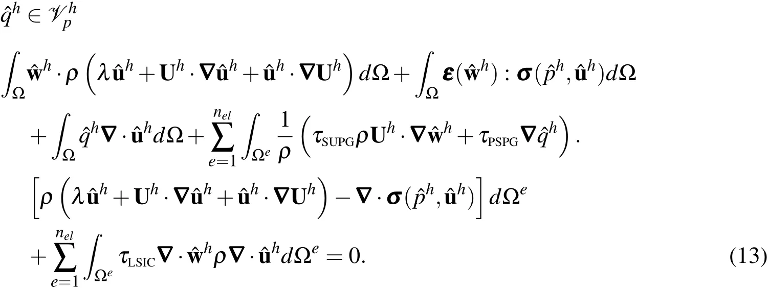
Here,Uhrepresents the base flow at the element nodes.In the variational formulation given by Eq.(13),the first three terms constitute the Galerkin formulation of the problem.The terms involving the element level integrals are the stabilization terms added to the basic Galerkin formulation to enhance its numerical stability.These terms stabilize the computations against node-to-node oscillations in advection dominated flows and allow the use of equal-in-order basis functions for velocity and pressure.The terms with coeffi cientsτSUPGand τPSPGare based on the SUPG(Streamline-Upwind/Petrov-Galerkin)[Brooks and Hughes(1982)]and PSPG(Pressure-stabilized/Petrov-Galerkin)[Tezduyar,Mittal,Ray,and Shih(1992)]stabilizations.The SUPGformulation for convection dominated flowswas introduced by Hughes and Brooks(1979)and Brooks and Hughes(1982).PSPG stabilization for enabling the use of equal-order interpolations for the velocity and pressureto fluid flowsat finite Reynoldsnumber wasintroduced by Tezduyar,Mittal,Ray,and Shih(1992).The term with coeffi cientτLSICis a stabilization term based on theleast squares of thedivergencefreecondition on the velocity field.It providesnumerical stability at high Reynoldsnumber.Here,thestabilization coefficients used in the finite element formulation of LSA(Eq.(13))are computed on the basis of the base flow at the element nodes,Uh.The stabilization parameters aredefi ned as[Tezduyar,Mittal,Ray,and Shih(1992)]:

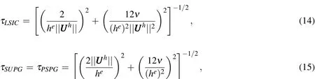
Here,heis the element length based on the minimum edge length of an element[Mittal(2000)]and Uhisthebase flow velocity at element nodes.

Eq.(13)lead to a generalized non-symmetric eigenvalue problem of the form A X−λB X=0.For our case,theeigenvalueproblem isslightly morecomplicated asthecontinuity equation responsiblefor determining pressurecausesthematrix B to becomesingular.Hence,to avoid singularity,wesolvetheinverseproblem,i.e.,eigenvalues for B X−µA X=0 are computed.Here,λ =1/µ.To check the stability of the steady-state solution we look for the rightmost eigenvalue(eigenvalue with largest real part),using thesubspaceiteration method[Stewart(1975)].

3.2 The Spectral Method for Local Linear Stability Analysis

Thespectral collocation method based on Chebyshev polynomialsof thefi rstkind[Schmid and Henningson(2001)]isused to solvethe Eq.(11)for carrying out thelocal sta-

bility analysis.The Chebyshev polynomial of the fi rst kind isdefi ned as:

for all non-negativeintegers n∈[0,N]and y∈[−1,1].By using asuitabletransformation,it ispossibleto map any other rangeof y to the Chebyshev domain[−1,1].The Chebyshev polynomials areutilized as the basis functions to approximate the eigenfunction,ˆv(y)in Eq.(8):

Thisapproximation of theeigenfunction issubstituted in the OSequation(Eq.(11).It resultsin the following equation:

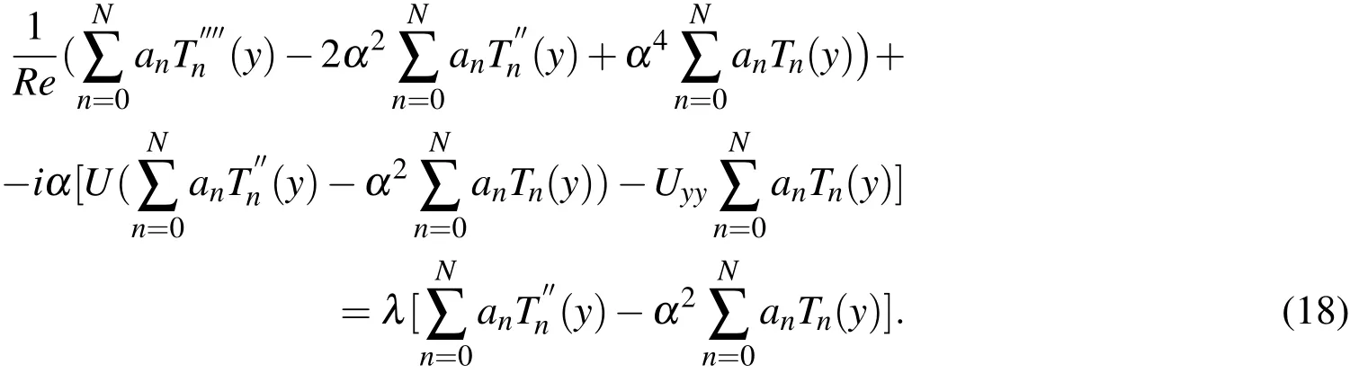
Thecollocation method isemployed to evaluatetheconstants anin theapproximation given by Eq.(17).The following Gauss-Lobatto collocation pointsareused:

Eq.(18)leads to the generalized eigenvalue problem of the form A X−λB X=0.In the present work,the numerical solution to the same is obtained using LAPACK[Anderson,Bai,Bischof,Blackford,Demmel,Dongarra,Du Croz,Greenbaum,Hammarling,McKenney,and Sorensen(1999)]libraries.

4 Problem Setup

4.1 The Base Flow

Thelocal and theglobal linear stability analysisarecarried outfor theplane Poiseuille flow.Figure(1)shows the schematic of the flow.The fluid occupies the channel formed by two stationary plates parallel to each other and separated by a distance 2H.Theplatesarealigned with the x−axis.Thevelocity profilefor thebaseflow

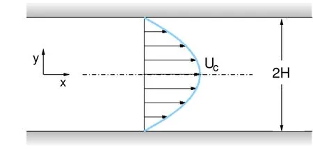
Figure1:Schematic of theplane Poiseuilleflow.

is shown in the fi gure.It is parabolic and symmetric about the channel centerline.The equation for the streamwise component of velocity isgiven as:

Here,H denotes half the channel width and Ucis the centerline velocity.All the lengthsarenon-dimensionalized with H,and velocity with Uc.The Reynoldsnumber,Re,isdefined as:

where,νdenotesthekinematic viscosity of thefluid.

4.2 Local Linear Stability Analysis

The local analysis of the plane Poiseuille flow iscarried out via the solution to OS(Eq.(11)).The domain across the channel width,[−H,H],is mapped to[−1,1].No-slip boundary conditions are applied to the disturbance fi eld at the channel walls.In thissituation,Eq.(12)can berewritten as:

The OSequation(Eq.(11)),along withtheboundary conditions(Eq.(22),issolved in thetemporal point of view.The wavenumber,α,is assumed to bereal.The OS equation is solved for different values of values ofαand Re.The effect of the number of grid points,along y,on the accuracy of the solution is investigated.It is found that 200 collocation points provide adequate spatial resolution.All the resultspresented in thispaper for the OSanalysisarewith 200 points.

4.3 Global Linear Stability Analysis

The flow in a fi nite streamwise length of the channel(=L)is considered for carrying out theglobal analysis.Thebaseflow isthefully developed steady flow in the channel.The streamwise velocity for the same is given by Eq.(20).The boundary conditions for thedisturbance fi eld are as follows.The disturbance velocity is prescribed a zero value at the upper and lower walls.To enable comparison with the local analysis,the disturbance is assumed to be periodic in the streamwise direction.Therefore,periodic boundary conditionsareapplied on all thevariablesat the inflow and theoutflow boundaries.Thefi niteelementmesh consistsof 24 elements alongthestreamwiseand 150elementsinthecross-flow directions.Thegrid points are uniformly spaced along x but are clustered close to the wall in the y direction.A mesh convergence study is carried out for the Re=7000 plane Poiseuille flow and L/2H=1.A more refi ned grid with roughly twice the resolution in each direction leadsto lessthan onepercentdifferencein theresults,thereby reflecting the adequacy of theoriginal fi nite element mesh.

5 Results:Linear Stability Analysisof the Plane Poiseuille Flow

5.1 OSAnalysis

Local analysis via solution to the OS equation(Eq.(11))is carried out for various values of Re andα.At each(Re,α)the eigenvalue with the largest real part is identified.Figure(2)shows the variation of the growth rate of the disturbance associated with the rightmost eigenvalue with Re andα.The fi gure shows the iso-contours for various values of growth rate in the Re−αplane.The contour corresponding to zero growth rateistheneutral curve.Thecritical Re for theonset of instability is the lowest value of the Re on the neutral curve,for any value of α.The critical Re for this flow is found to be 5773,approximately and is marked in Figure(2).The value is in excellent agreement with results from earlier studies[Schmid and Henningson(2001)].

Theresultsfor theflow at Re=7000 arepresented inmoredetail in Figure(3).This fi gureshowsthevariation of thereal(λr)and imaginary(λi)partsof therightmost eigenvalue with wavenumber(α)at Re=7000.While λrdenotes the growth rate,λiis related to the temporal frequency of the disturbance.We observe that the Re=7000 flow is linearly unstable only to disturbances whose wavenumber lies in a specifi c interval.The maximum growth rate is0.0017,approximately forα=1.00.

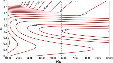
Figure 2:Orr-Sommerfeld analysis of the Plane Poiseuille flow:iso-contours of constant growth rate.The critical Re for the onset of the instability of the flow is Recr=5773 and ismarked with a vertical broken line.

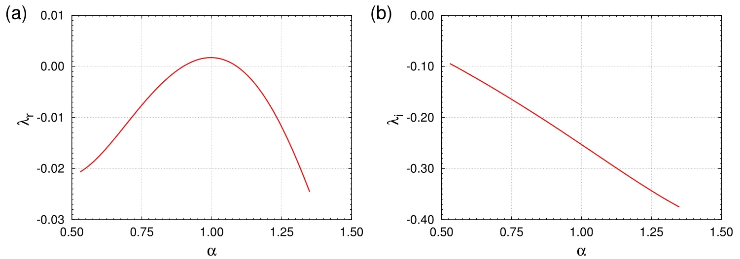
Figure 3:Orr-Sommerfeld Analysis of the Plane Poiseuille Flow at Re=7000:variation of real and imaginary partof theright-most eigenvaluewith wavenumber,α.

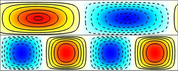
Figure 4:Global linear stability analysis of the Plane Poiseuille flow for Re=7000 and L/2H=5.10:the v′field for the eigenmodes corresponding to the two rightmost eigenvalues.The upper row corresponds to one cell in the domain(n=1)and has a growth rate,λr=−0.017.The lower row is for n=2 with two cells in thedomain;the growth ratefor this mode isλr=−0.0097.

5.2 Global Analysis

In thelocal analysis,the OSequation(Eq.(11))can besolved by usingαasoneof the independent variables.However,the global analysis(Eq.(6))does not directly offerαas an independent variable.The analysis,of course,can be carried out for different streamwise extent(L)of the computational domain.We attempt to understand the relation between L(for the global analysis)andα(for the local analysis).We propose that for a spatially periodic disturbance,its wavenumber is related to thelength of thecomputational domain as:

where,n is the number of waves along the stream wise direction in the domain.To demonstratethis,weconsider theglobal linear stability analysisfor Re=7000.Fig.(4)shows the eigen modes associated with the two right most eigenvalues for L/2H=5.1.While the first one is associated with one wave(n=1),the other houses two waves(n=2)in the computational domain.Thus,they both represent different wavenumbersand areassociated with their own growth rates,aslisted in the caption of the fi gure.The real and imaginary part of the eigenvalue obtained from the global analysis,and their comparison with the values obtained from the local analysis,arealso shown in Figures(5)and(6).Thedatapointscorresponding to the two eigenmodes lie on the vertical line segment marked in the two figures for L/2H=5.10.The values from the local and global analysis are in excellent agreement.

Figures(5)and(6)show the variation of the growth rate and the imaginary part of the rightmost eigenvalue from the global analysis for plane Poiseuille flow at Re=7000.The data points from the global analysis are marked by solid circles.Also shown in thesamefigurearetheresultsfrom thelocal analysis.Thevariation is associated with a number of peaks and valleys.We attempt to understand this behavior.It isdemonstrated in Fig.(4)that thecomputational domain may accommodate multiple cells of the disturbance.We fi rst identify in Figs.(5)and(6)the cases that are associated with onecell only(n=1)in thestreamwise extent of the domain.A best fi t to these points is in excellent agreement with the results from the local analysis.These curves are marked as L=2π/α in the figures.These curvescan also beutilized to understand thevariation ofλrandλiwithα.Wenote that thegrowth rateand temporal frequency of an eigenmodeshould depend onα,but must beindependent of thenumber of cellsof the sameαin the computational domain.Usingthisidea,and thedataforλrandλiv/sα fromthelocal analysis,the variation ofλrand λiwith L/2H is generated for multiple cells by observing that L=2πn/α,where n is the number of cells.These curves are shown in Figs.(5)and(6)for various values of n.The outer envelope of these curves is shown in thicker solid line.These curves provide an estimate of the variation of the rightmost eigenvaluewiththelength of thecomputational domain.Excellentagreement is observed between the estimated rightmost eigenvalue and the actual value from global LSA computationsfor n≥2.Wenotethatasthelengthof thecomputational domain isincreased,thedependenceof the growth rateof themost unstableeigenmodeon L becomesweaker.In theasymptotic limit of thedomain being infinitely long,the fastest growing mode comprises of infi nite cells of the n=1 eigenmode whose wavenumber is associated with largestλr.We also note from Fig.(5)that in certain situations it might be diffi cult to track the eigenmodes corresponding to low values ofαfrom the global analysis.Low values ofα correspond to large L/2H.Asseen from Fig.(5),at large L/2H,n=1 modeisnot necessarily theone with rightmost eigenvalue.For example,at L/2H=15 the rightmost eigenvalue corresponds to the mode with five cells(n=5).The modes with four,three,two and onecell have lower growth rate,and in the sameorder.Therefore,tracking the modefor n=1 for thisvalueof L/2H is relatively morechallenging than theones for higher valuesof n.

To further demonstrate that the growth rate and temporal frequency of an eigenmode must be independent of the number of streamwise cells in the global analysis,weconsider thecasewhereweseek therightmost eigenvalueforα=1.05.For n=1,thiscorrespondsto L/2H=3.0,approximately.Figure(7)showstheeigenmodesfromtheglobal analysisfor variousvaluesof L/2H for thesameα(=1.05).Thevariousvaluesof L arechosen by varying n in therelation L=2 nπ/α.A broken horizontal lineismarked in Figures(5)and(6)to show thereal and imaginary partof therightmosteigenvaluefor variousvaluesof L thatcorrespond toα=1.05.We observe that all these modes are associated with the same eigenvalue.In fact,theeigenmodesarealso of thesamefamily.They areshown in Figure(7)and have

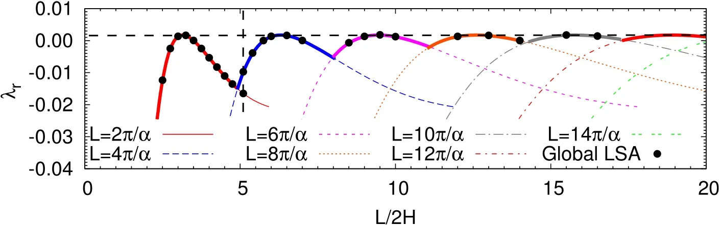
Figure 5:Variation of the growth rate of the leading eigenvalue with L/2H for the plane Poiseuilleflow for Re=7000:thesolid dotsrepresent thegrowth rateof the mostunstablemodeobtained atvariousvaluesof L/2H fromglobal LSA.Thesolid(red)curveisobtained from thelocal(Orr-Sommerfeld)analysis.It isin excellent agreement with the best fi t to the points corresponding to one streamwise wave(n=1)from global analysis asper the relation L=2π/α.The curve isreplicated for various n to show the predicted variation ofλr with L,for the global analysis using the relation L=n(2π/α),when the domain houses different number of cells.Theouter envelopeof thesecurves,showninthicker solid line,representsthe eigenmode associated with the rightmost eigenvalue for the corresponding length of thecomputational domain.

the sameflow structure,albeit with different number of cells.

6 Concluding Remarks

Hydrodynamic stability of shear flows has been widely investigated in the past usinglocal and global Linear Stability Analysis(LSA).Inthiswork wehavereviewed thetwo approachesand attempted to highlightthedifferencebetween thetwo in the context of their application to parallel shear flows.Resultsfor thelinear stability of plane Poiseuille flow have been presented,using both approaches.The local analysisiscarried out by solving the Orr-Sommerfeld(OS)equation using thespectral collocation method based on Chebyshev polynomials.The analysis has been carried out for various wavenumbers,αof the streamwise periodic disturbance fi eld.The critical Re for the onset of linear instability for plane Poiseuille flow is found to be 5773,which is in good agreement with earlier results[Schmid and Henningson(2001)].The stability of the flow at Re=7000 has been presented in more detail.For example,the variation of the real and imaginary part of the least stable eigenvalue withαhas been presented.Unlike the local analysis which involves solution to an ordinary differential equation,the global analysis involves fi nding solution to a set of partial differential equations.The analysis has been carried out for atwo-dimensional disturbance fi eld that isassumed to bespatially periodic along the stream wise direction.A stabilized finite element method has been presented for carrying out the global LSA in primitive variables.Equal-in-order fi nite element functions are used for representing velocity and pressure.To suppress the numerical oscillationsthat might appear in thecomputations,the SUPGand PSPG,stabilizationsareadded tothe Galerkinfiniteelementformulation.Theformulation hasbeen used to carry out the linear stability analysisfor the plane Poiseuille flow at Re=7000.Computations are carried out for various values of the streamwise length,L,of thecomputational domain.

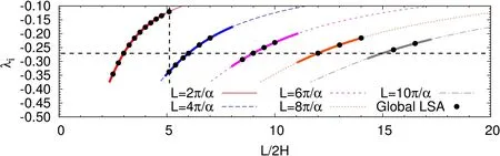
Figure 6:Variation of the imaginary part of theleading eigenvalue with L/2H for theplane Poiseuilleflow for Re=7000:thesolid dotsrepresent theimaginary part of the most unstable mode obtained at various values of L/2H from global LSA.The solid(red)curve isobtained from the local(Orr-Sommerfeld)analysis.It isin excellent agreement with thebest fit to thepointscorresponding to onestreamwise wave(n=1)from global analysis as per the relation L=2π/α.The curve is replicated for various n to show the predicted variation ofλi with L,for the global analysisusingtherelation L=n(2π/α),when thedomainhousesdifferent number of cells.The curves shown in thicker solid line representsλi associated with the rightmost eigenvaluefor thecorresponding length of thecomputational domain.

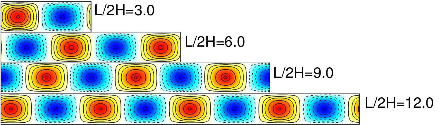
Figure 7:Eigenmodes of v′corresponding to the leading eigenvalue for various lengths of the domain obtained with the global LSA for the plane Poiseuille flow for Re=7000 for disturbancesthat areperiodic in thestreamwise direction.

Unlike the local analysis, the global analysis can handle non-periodic disturbances and is applicable to non-parallel flows as well. However, the global analysis is signifi cantly more expensive than the local a nalysis. For the parallel flow and with spatially periodic disturbances the present work brings out a very interesting relationship between the wave number of the disturbance and the streamwise extent of the domain in the global analysis. When the eigenmode contains only once cell, the results from the local and global analysis are virtually identical; the wavenumber and streamwise extent of the domain are related as α = 2 π/L. However, when the eigenmode consists of n cells along the streamwise length of the domain the relationship is: α = (2 πn)/L. For a very large value of L, the global analysis results in an eigenmode with a large number of cells of the eigenmode whose α corresponds to the mode with largest growth rate. If one would like to use the global analysis to create the growth rate v/s α curve for the rightmost eigenvalue, as is done in the local analysis for a specific value of Re, the procedure is complicated by the number of cells that are housed in the domain. In the scenario when L is relatively large, to track an eigenmode for low α, the eigenmode associated with one cell might not be the most unstable mode. Therefore, one needs to examine the eigenmodes for the first few eigenvalues that are arranged in the descending order of their real part.The one that corresponds to α = 2 π/L is the eigenmode which consists of only one cell along the streamwise direction.

Acknowledgement:The help from Mr.Hardik Parwana in carrying out some of thecomputationsisgratefully acknowledged.

Anderson,E.;Bai,Z.;Bischof,C.;Blackford,S.;Demmel,J.;Dongarra,J.;Du Croz,J.;Greenbaum,A.;Hammarling,S.;McKenney,A.;Sorensen,D.(1999):LAPACKUsers’Guide.Society for Industrial and Applied Mathematics,Philadelphia,PA,third edition.

Boiko,A.V.;Dovgal,A.V.;Grek,G.R.;Kozlov,V.V.(2012): Physics of Transitional Shear Flows.Springer-Verlag.

Brooks,A.;Hughes,T.(1982):Streamlineupwind/petrov-galerkin formulations for convection dominated flows with particular emphasis on the incompressible navier-stokes equations.Computer Methods in Applied Mechanics and Engineering,vol.32,pp.199–259.

Chandrasekhar,S.(1981): Hydrodynamic and hydromagnetic stability.Dover.

Chomaz,J.-M.(2005): Global instabilities in spatially developing flows:nonnormality and nonlinearity.Annual Review of Fluid Mech.,vol.37,pp.357–392.

Chomaz,J.M.;Huerre,P.;Redekopp,L.G.(1988):Bifurcations to local and global modes in spatially developing flows.Physical Review Letters,vol.60,pp.25–28.

Davey,A.;Drazin,P.(1969):Thestability of poiseuilleflow in apipe.J.Fluid Mech.,vol.36,pp.209–218.

Garg, V. K.; Rouleau, W. T. (1972): Linear spatial stability of pipe poiseuille flow. J. Fluid Mech., vol. 54, pp. 113–127.

Gaster,M.(1962): A note on the relation between temporally-increasing and spatially-increasing disturbances in hydrodynamic stability.J.Fluid Mech.,vol.14,pp.222–224.

Huerre,P.(2000): Open shear flow instabilities.In Batchelor,G.;Moffatt,H.;Worster,M.(Eds):Perspectivesin Fluid Dynamics,pp.159–229.Cambridge.

Huerre,P.;Monkewitz,P.(1990): Local and global instabilities in spatially developing flows.Annual Review of Fluid Mech.,vol.22,pp.473–537.

Hughes,T.;Brooks,A.(1979): A multi-dimensional upwind scheme with no crosswind diffusion.Journal of Applied Mechanics,vol.34,pp.19–35.

Jackson,C.(1987):A fi niteelement study of theonset of vortex shedding in flow past variously shaped bodies.J.Fluid Mech.,vol.182,pp.23.

Mittal,S.(2000): On the performance of high aspect-ratio elements for incompressible flows.Computer Methods in Applied Mechanics and Engineering,vol.188,pp.269–287.

Mittal,S.(2004):Three-dimensional instabilitiesin flow past a rotating cylinder.Journal of Applied Mechanics,vol.71,pp.89–95.

Mittal,S.;Kumar,B.(2003): Flow past a rotating cylinder.Journal of Fluid Mechanics,vol.476,pp.303–334.

Monkewitz,P.A.(1988): The absolute and convective nature of instability in two-dimensional wakes at low Reynolds numbers.Physics of Fluids,vol.31,pp.999–1006.

Morzynski, M.; Afanasiev, K.; Thiele, F. (1999): Solution of the eigenvalue problems resulting from global non-parallel flow s ta bility analysis.Comput. Meth-ods Appl. Mech. Eng., vol. 169, pp. 161.

Morzynski,M.;Thiele,F.(1991):Numerical stability analysis of aflow about a cylinder.Z.Angew.Math.Mech.,vol.71,pp.T424.

Navrose;Meena,J.;Mittal,S.(2015): Three-dimensional flow past a rotating cylinder.J.Fluid Mech.,vol.766,pp.28–53.

Orr,W.M.(1907):The stability or instability of the steady motions of a perfect liquid and of a viscousliquid.Proc.R.Irish Acad.Sec.A,vol.27,pp.9–138.

Orszag,S.A.(1971):Accurate solution of the orr-sommerfeld stability equation.J.Fluid Mech.,vol.50,pp.689–703.

Pierrehumbert,R.T.(1985): Local and global baroclinic instability of zonally varying flow.Journal of the Atmospheric Sciences,vol.41,pp.2141–2162.

Saraph,V.;Vasudeva,B.R.;Panikar,J.(1979):Stability of parallel flowsby the fi nite element method.Int.J.Numer.Methods Engineering,vol.17,pp.853–870.

Schmid,P.J.;Henningson,D.S.(2001): Stability and Transition in Shear Flows.Springer-Verlag.

Sommerfeld,A.(1908):Ein Beitrag zur hydrodynamischen Erkläerung der turbulenten Flüessigkeitsbewegungen. Proc.Fourth Internat.Cong.Math.,Rome,vol.III,pp.116–128.

Stewart,G.(1975):Methods of simultaneous iteration for calculating eigenvectors of matrices.In Miller,J.(Ed):Topics in Numerical Analysis II,pp.169–185.Academic Press:New York.

Swaminathan,G.;Sahu,K.;Sameen,A.;Govindrajan,R.(2011): Global instabilities in diverging channel flows.Theor.Comput.Fluid Dyn.,vol.25,pp.53–64.

Tezduyar,T.;Mittal,S.;Ray,S.;Shih,R.(1992):Incompressibleflow computations with stabilized bilinear and linear equal-order-interpolation velocity-pressure elements.Comput.Meth.Appl.Mech.Engrg,vol.95,pp.221.

Theofilis,V.(2011):Global linear instability.Annual Review of Fluid Mech.,vol.43,pp.319–352.

Verma,A.;Mittal,S.(2011): A new unstable mode in the wake of a circular cylinder.Phys.Fluids.,vol.23,pp.121701.

Yang,X.;Zebib,A.(1989): Absolute and convective instability of a cylinder wake.Physicsof Fluids A,vol.1,pp.689–696.