Modern methods for longitudinal data analysis, capabilities,caveats and cautions

Lin GE, Justin X. TU, Hui ZHANG, Hongyue WANG, Hua HE, Douglas GUNZLER

•Biostatistics in psychiatry (35)•

Modern methods for longitudinal data analysis, capabilities,caveats and cautions

Lin GE1, Justin X. TU2, Hui ZHANG3, Hongyue WANG1, Hua HE4, Douglas GUNZLER5

binary variables, correlated outcomes, generalized linear mixed-effects models, weighted generalized estimating equations, latent variable models, R, SAS

1. Introduction

Longitudinal study designs have become increasingly popular in research and practice across all disciplines.Such designs capture both between-individual differences and within-subject dynamics, providing opportunities to study complex biological, psychological and behavioral changes over time such as causal treatment effects and mechanisms of change[1,2]. Since longitudinal study designs create serial correlations over repeated assessments from same subjects, traditional statistical methods for cross-sectional data analysis such as linear and logistic regression do not apply. In addition, since longitudinal studies are typically of long duration, missing data is common. Specialized models and methods must be used to address the two major issues.

The two dominant approaches for longitudinal data analysis are the generalized linear mixed-effects model (GLMM) and weighted generalized estimating equations (WGEE)[1]. Both methods are derived from the same class of models for cross-sectional data, the generalized linear models (GLM). Because different techniques are used to extend the GLM to longitudinal data, the GLMM and WGEE are quite different and some of the differences carry significant implications for their applicability and interpretation of study findings.Despite the existence of an extremely large body of literature discussing the development and application of the two approaches, practitioners still often face many difficult questions when choosing and applying such models to real study data.

For example, which approach is applied given data from a study? Do the two approaches yield identical estimates and/or inferences? If not, how should one approach and interpret such differences? What are the pros and cons associated with each approach? Although some questions have well-documented answers in the literatures, others have only been approached recently and still await answers.

In this report, we first give an overview of the approaches and then discuss major differences between the two classes of models. Unlike the literature on the discussion of the two methods, we focus on their practical implications, which we think provide useful guidance for practitioners for selecting right approaches for their studies and effectively addressing their study questions.

2. Models for Longitudinal Data

Since both the GLMM and WGEE are extensions of the GLM, we start with a brief overview of the latter.

2.1 Generalized Linear Models (GLM)

Consider a sample of n subjects and let Yi(Xi) denote a continuous response (a vector of explanatory variables).The classic linear model is given by:

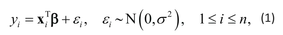
where N(μ, σ2) denotes a normal distribution with mean μ and σ2variance. The linear model is widely used in research and practice. One major limitation is that it only applies to continuous response Yi. The generalized linear models (GLM) extend the classic linear model to non-continuous response such as binary.

To express the GLM, we first rewrite the linear regression in (1) as

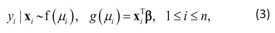
where f(μ) denotes some distribution with mean μ and g(μ) is a function of μ. Since g(μ) links the mean to the explanatory variables, g(μ) is called the link function.

The specification of f(μ) and g(μ) depend on the type of response Yi. For a binary Yi, f(μ) is the Bernoulli distribution and g(μ) is often set as the logit function

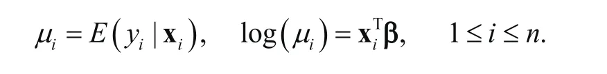
The resulting GLM is the logistic regression. For a count Yi, a popular choice for f(μ) is the Poisson distribution and g(μ) is the log function, g(μ) =log(μ).Another choice for f(μ) is the negative binomial. A major limitation of Poisson is that its variance is the same as its mean. Count responses arising in many real studies often have variances larger than means, a phenomenon known as “overdispersion”[1].The negative binomial is similar to the Poisson, but unlike the Poisson, allows for overdispersed count responses[1].

Inference for GLM can be based on maximum likelihood (ML) or estimating equations (EE). The classic ML provides most efficient estimates, if the response Yifollows the specif i ed distribution such as the normal in the linear regression in (1). In many studies, it may be difficult to specify the right distribution, in which case the ML will yield biased estimates if the specif i ed distribution does not match the data distribution. The modern alternative EE uses an approach for inference that does not require specification of a mathematical distribution forYi, thereby providing valid inference for a wider class of data distribution. Since no distribution is required under EE, we may also express the GLM in this case as:

or simply

or equivalently

Example 1. In a suicide study, we may model number of suicide attempts, Yi, a count response, using a parametric GLM:

where Xidenotes a set of explanatory variables such as age, physical problems and history of depression.If concerned about overdispersion, such as indicated empirically by a much larger variance as compared to the mean, the semi-parametric GLM below may be used

Unlike the parametric model in (7), the semi-parametric GLM above provides valid inference regardless of presence of over-dispersion.

2.2 Extension of GLM to longitudinal data

1.1.1 Weighted Generalized Estimating Equations(WGEE)

Consider a longitudinal study with T time points and let Yitand Xitdenote the same response and predictors/covariates as in the cross-sectional setting, but with t indicating their dependence on the time of assessmentFor each time t , we can apply the GLM in(3) to model the regression relationship between Yitand Xitat each point

We can then get estimates of βtfor each time point t. However, it is difficult to interpret different βtacross the different time points. Moreover, it is technically challenging to combine estimates of βtto test hypotheses concerning temporal trends because of interdependence between such estimates.

The WGEE addresses the aforementioned difficulties by using a single estimate β to model changes over time based on multiple assessment times[1,3]. Since the WGEE estimates β using a set of equations that do not reply on assumed distribution ( )fitµ in (8), the first part of the GLM can be removed and the resulting model becomes

By comparing the WGEE above with the model in (4), it is seen that the WGEE is an extension of the semi-parametric GLM to longitudinal data. The key difference between (4) and (8) is that (8) is not simply an application of GLM to each of the time points, but rather an extension of the model in (4) to provide a single parameter vector β for easy interpretation and estimate this parameter vector by using data from alltime points and accounting for correlations between the repeated assessments. Like the semi-parametric GLM,the WGEE provides valid inference for a wider class of data distributions.

2.3 Generalized Linear Mixed-effects Models (GLMM)

The GLMM extends the GLM to longitudinal data analysis using a completely different approach.

Consider again a longitudinal study with T time points and let Yitand Xitdenote the same response and predictors/covariates as in the WGEE above. The GLMM is specif i ed by:

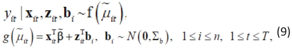
Unlike the WGEE, the GLMM accommodates correlated responses Yitby directly modeling their joint distribution. Since multivariate distributions are extremely complex except for the multivariate normal,latent variables biare generally employed to model the correlated responses. Thus, although Yitis still modeled for each time point t, by including the random effect biin the specification of the conditional distribution of Yitgiven bi(Xitand Zit), the GLMM in (9) allows the resulting Yit’s to be correlated (conditional on Xitand Zitonly). This approach allows one to specify multivariate distributions using familiar univariate distributions such as the Bernoulli (for binary responses) and the Poisson(for count responses).

2.4 Key differences between GLMM and WGEE

Although both WGEE and GLMM are extensions of the GLM, the two approaches are quite different because of the way the extensions are accomplished. In this section, we discuss such key differences.

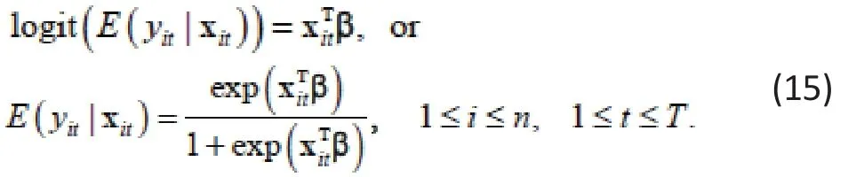
2.4.1 Interpretation of Model Parameters

A fundamental difference between the WGEE and GLMM is in interpretation of model parameters. As noted earlier, the WGEE is an extension of the semiparametric GLM, while the GLMM is an extension of the parametric GLM. Although the parameter vector β has the same interpretation between the parametric (1)and semi-parametric (4) GLM, the parameter vectors β in the WGEE (8) and β in the GLMM (9) are generally different except for the linear regression.

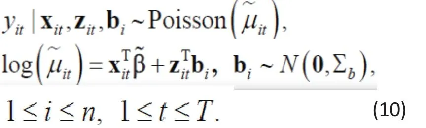
Example 2. Consider the model in Example 1, but now assume a longitudinal study with T assessment times.Let Yitand Xitdenote the longitudinal versions of Yiand Xi. Again, if Yitat each point is modeled to follow a Poisson, the GLMM has the form:

On the other hand, the WGEE for a count response has the form

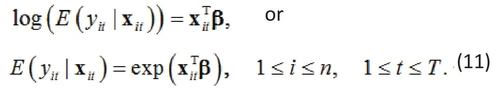
The two models look quite the same, except for the additional random effect in (10). So, to compare the two models, we integrate out biin (10) and calculate the conditional expectationto obtain (see Zhang et al., 2012 for derivation)[4]

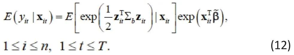
This conditional expectation is different from the expression in (11) for the WGEE unless

In some special cases, β andmay be identical except for the intercept term. For example, ifis independent of, then

Thus (12) reduces to

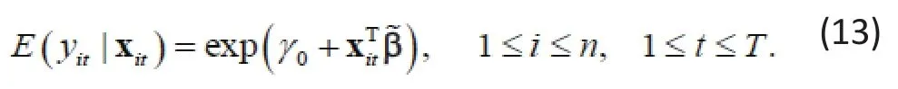
Except for the intercept term, β andhave the same interpretation. The next Example illustrates this special case with data from a real study.

Example 3. The COMBINE study was a multi-site randomized clinical trial with longitudinal followup to compare intervention effects between nine pharmacological and/or psychosocial treatments. For illustration purposes, we combined all the 9 treatment conditions and focused on the two drinking outcomes,days of any drinking and days of heavy drinking over the past month, at three visits during treatment at weeks 8,16 and 26.

Since Zi=1 and Xi1t=1 are both constants, they are independent. We fi t a WGEE with the same predictors Xit=(Xi1t,Xi2t,Xi3t)Tas in the fixed effect of GLMM above.As indicated in Example 2,differs from its WGEE counterpart β0by a constant, whereasandretain the same scales as the corresponding β1and β2in the WGEE model.

Shown in Table 1 are the estimates of β andand associated standard errors, and test statistics and associated p-values for both models. As expected,estimates ofandwere quiteclose to the respective WGEE estimates β1and β2, but those of were much smaller (in magnitude) than their WGEE counterparts (0.694 vs. 1.908 for Days of Any Drinking and -0.30 vs. 1.307 for Days of Heavy Drinking).Sinceand(β1and β2) represent changes relative to the reference level(β0) from Visit 1 to Visit 2 and from Visit 1 to Visit 3 under GLMM (WGEE), the difference between the estimatedand β0implies not only different means at visit 1, but also at visits 2 and 3 for each drinking outcome. For example, for the outcome of Days of Any Drinking, the WGEE estimates indicate a mean of 6. 7, 7.7 and 8.9 days of any drink over the three visits, much lower than 1.9, 2. 3 and 2.7 days of any drink at the corresponding visits estimated by the GLMM. The WGEE estimates are actually identical to sample means of this drinking outcome at each visit, but the GLMM estimates are not, making the latter difficult to interpret.

Table 1. Estimates of reference level at Visit 1 (β ̃0 for WGEE and β0 for GLMM) and change from reference level at Visit 2 (β1 and β ̃1)and at Visit 3 (β2 and β ̃2), along with associated standard errors, for Days of Any Drinking and Days of Heavy Drinking for the real COMBINE Study in Example 3.

Example 4. In Example 2, now suppose thatity is binary and is modeled by a GLMM for binary response as follows

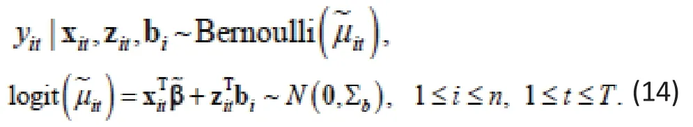
The corresponding WGEE has the form

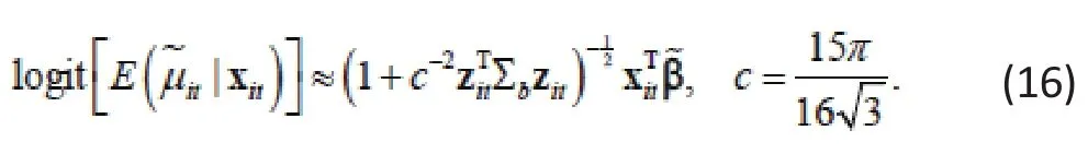
As in Example 2, the two models look the same, except for the additional random effect in (14). To compare the two, we again need to integrate out biin (14). In general, it is difficult to obtain a closed-form expression for the resulting integral. But, in the special case when Zitis a subset of Xitand Zit=Zt, the integral can be expressed as (see Zhang, Xia et al., 2011 for derivation)[5]Thusis a rescaled β. Even in this special case, it may not easy to interpret,as demonstrated by a real study example next.

Example 5. In a recent study on smoking cessation,276 subjects participated in multi-component program adapted to seriously mentally ill patients within an outpatient mental health clinic. Out of these subjects,99 also participated in a formal evaluation, in which interviews were conducted at the point of enrollment(baseline) and again at 3, 6 and 12 months. A primary outcome of the study is the 7-day point prevalence abstinence (defined as no smoking at all in the previous 7 days). We modeled changes of this longitudinal binary abstinence outcome using data from the 99 subjects.

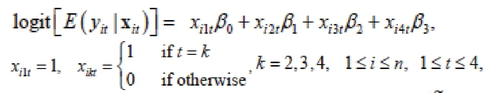
We applied both longitudinal approaches and used three dummy variables to model the rate of 7-day point prevalence abstinence at each of the follow-up times for the WGEE and also included a random intercept for the GLMM model. Thus, the GLMM has the form

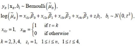
while the WGEE is given by:

Shown in Table 2 are the estimates of β andand associated standard errors, and test statistics and associated p-values for both models. The estimates were quite different between the two models, although the ratio, a constant for all 1＜k＜3. This is not a coincidence, but expected, because of (16) and the fact that Zitiin the GLMM model is a subset of Xit.Also, sinceunder one model implies that holds true for the corresponding coefficient under the other model, same conclusions were obtained regarding statistical significance of the parameters, although the p-values under the two models were slightly different.The scale difference in the parameters between the two models did have serious implications for the interpretation of estimates from the GLMM. Shown in the last two columns of Table 2 are the rates of 7-day point prevalence abstinence over time estimated by each of the two models. Since the WGEE becomes the logistic regression at each assessment time, it yields estimates identical to the observed rates of 7-day point prevalence abstinence. Estimates from the GLMM were quite different, underestimating the observed rates by over 50%. Even in this simplest case where estimates of GLMM are a scale shift of their GEE counterparts,GLMM estimates are difficult to interpret.

2.4.2 Computational Issues for GLMM

Inference for the WGEE is based on a set of equations.Although it is generally not possible to express solutions (estimates) in closed-form, the equations are readily solved numerically[1]. Inference for the GLMM, however, is much more challenging. Since the likelihood function arising from the GLMM is generally quite complex, involving multidimensional integrals,it is difficult to directly maximize this function except for the special linear models case for continuous outcomes. Different approaches have been proposed to address the computational issues when modeling noncontinuous responses using the GLMM.

The approach implemented in most major software such as SAS and R is integral approximation. This approach fi rst approximates the log-likelihood function and then maximizes the approximated function using the Newton and Gauss-Hermite quadratures. However,studies have shown that the approach does not work well as one would expect[6], especially for modeling binary responses. Below, we highlight some key findings from these studies.

Example 6. Zhang, Lu and Feng et al. (2011)[6]examined the computational issues by fitting GLMM for simulated binary responses using both SAS and R. They simulated an explanatory variable Xiand the response Yitfrom the GLMM:

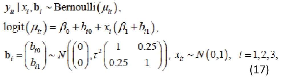
where β0=β1=1 and τ=0.001 and 2. For τ=0.001 , the within-subject correlation was very small and thus negligible, making theYit’s almost independent. For τ=2 ,the within-subject correlations was about 0.5.

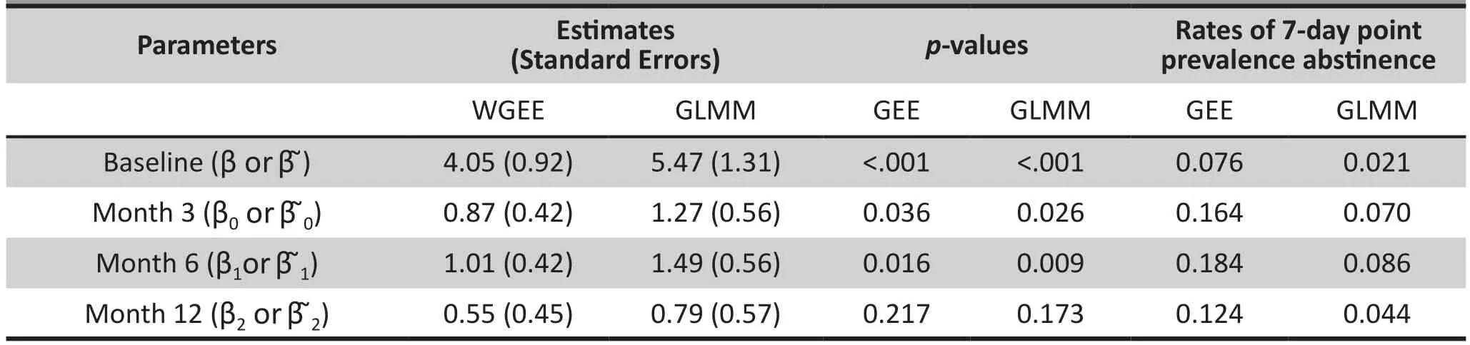
Table 2. Estimates of parameters, standard errors, p-values and rates of 7-day point prevalence abstinence at baseline and 3 follow-up visits from the WGEE and GLMM models for the real Smoking Cessation Study in Example 5.

They simulated data from the GLMM in (17) with a sample size n=500, fi t the same model to the simulated data using R and SAS, and repeated the process 1,000times. Shown in Table 3 are the estimates of parameter vector β (under “β0=1” and “β1=1” based on averaging over 1,000 estimates from fitting the model to each simulated data) and associated standard errors (under S.E.10× based on sample standard deviations from the Monte Carlo 1,000 estimates of β) from fitting SAS NLMIXED procedure and R lme4 function. For τ=0.001,the estimates were quite similar between the two, but for τ=2, the SAS NLMIXED procedure provided more accurate estimates. There were more pronounced differences in the standard errors between the two,with the R lme4 consistently yielding lower standard errors than the SAS NILMIXED. Such differences play a significant role in hypothesis testing.

Shown in Table 3 under “Type I error” are the type I error rates for testing the hypothesis,based on the Wald statistic from the SAS and R procedures. The Wald statistic is whereis the standard error for the estimate . The type I error rate was calculated as:

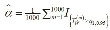
where q1,0.95is the 95th percentile ofanddenotes the Wald statistic for testing the hypothesis based on mth simulated dataSince the null hypothesisis true, the type I error rateshould be close to the nominal value α=0.05,if the SAS and R procedures provided correct inference.Although the SAS NLMIXED did yield type I error rates close to the nominal value, R lme4’s estimates were inflated, especially for the case with higher withinsubject correlation τ=2.

In addition to the SAS and R procedures, Zhang,Lu and Feng et al. (2011)[6]also considered other procedures in SAS and R and found that none provided correct estimates. Their conclusion was that the SAS NLMIXED procedure provided more accurate estimates and type I error rates. However, more recent studies by Chen, Knox, Arora et al. (2016)[7]and Chen, Lu, Arora et al. (2016)[8]show that this SAS procedure did not provide correct estimates either.

Table 3. Estimates of parameters, standard errors,Type I error rates (for testing null: H0: β1=1 from SAS NLMIXED and R lme4 procedures for two within-subject correlation cases (τ=0.001 and τ=0.0001 ) for the simulation study in Example 6.

Example 7. Chen, Knox, Arora et al. (2016)[7]considered clustered binary responses arising from multi-center studies. They modeled and simulated clustered binary responses from the following GLMM

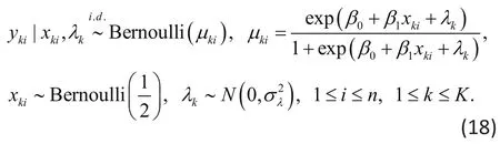
where K denotes the number of study sites, n number of subjects within each site (cluster size),kix is a binary variable indicating treatment condition assigned to the ith subject within the kth site, andkλ is the random effect accounting for correlations between responseskiy from subjects with the kth site. They considered testing the hypothesis:

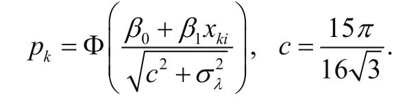
Chen, Knox, Arora et al. (2016)[7]consideredandwithclusters andwithin each cluster. For each, they obtained0β and β1and simulated data from the GLMM in (18)underThey fi t the model (18) to the data generated using SAS NLMIXED, tested the nulland rejected the null if the p-value is larger than α=0.05. The process was repeated 1,000 times and power was estimated by the percent of times the null was rejected.

Shown in Table 4 are power estimates under“NLMIXED” for the three cases ofalong with true power values under (“True”) obtained using a different approach developed in Chen, Knox, Arora et al. (2016)[7].As seen, power estimates from obtained from the SAS NLMIXED were quite different from the true power for each case of, all underestimating the true power.Note that when, there is no data cluster and power only depends on the total sample size Kn. In this case, we can also obtain power estimates by using instead the SAS LOGISTIC NLMIXED for non-clustered data. This is indeed the case, since Chen, Knox, Arora et al. (2016)[7]reported that they obtained power estimates similar to 0.561 when running the Monte Carlo substitution to estimate power using the SAS LOGISTIC.

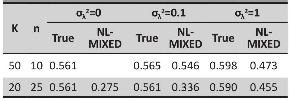
Table 4. Power estimates from SAS NLMIXED along with true power values for two data clustering cases (σλ2=0.1 and σλ2=1) for the simulation study in Example 7.

3. Discussion

In this report, we discussed the two most popular regression models for longitudinal data. We focused on interpretation and computation of model parameters.For parameter interpretation, we discussed differences between the GLMM and WGEE when applied to model binary and count responses. Since parameters from the two longitudinal models are generally quite different,we should not expect similar estimates when applying the two models to real study data. Moreover, except for some special cases, it is generally not possible to find a relationship between estimates from the two models.Our analysis indicates that GLMM estimates can be quite difficult to interpret, while WGEE estimates afford straightforward interpretation.

Another major issue with the GLMM is to obtain reliable estimates using existing software. It seems that even software giants like SAS cannot provide correct estimates when applying GLMM to model binary responses. Until the computational problem is resolved,one may want to consider applying WGEE when modeling longitudinal binary responses.

We focused on the binary and count response when discussing interpretation of model parameters in this report. When modeling continuous responses, the two longitudinal models have the same interpretation for their model parameters and thus the interpretational issue does not arise. The computational problem seems only relevant to binary responses. For continuous responses, the log-likelihood function can be solved accurately[1]. For count responses, major software such as R and SAS seem to provide quite reliable estimates.

Funding

The work was supported in part by a grant from NIH/NCRR CTSA KL2TR000440. The funding agreement ensured the authors’ independence in designing the study, interpreting the data, writing, and publishing the report.

Conflict of interest statement

The authors report no conflict of interest related to this manuscript.

Authors’ contributions

All authors worked together on the manuscript and contributed their expertise to the relevant sections.

Mr. Lin and Dr. Gunzler outlined the structure of the manuscript and integrated sections from the other authors.

Mr. Lin also performed some of the simulations under the supervision of Dr. Gunzler and Dr. Zhang.

Mr. Tu helped develop the real data examples and interpretation of results with Dr. Zhang, Dr. Wang and Dr. He helped develop the sections on longitudinal models and interpretation of simulation study results.

1. Tang W, He H, Tu XM. Applied Categorical and Count Data Analysis. Boca Raton, FL: Chapman & Hall/CRC; 2012

2. Gunzler D, Lu N, Tang W, Wu P, Tu XM. A Class of Distribution-free Models for Longitudinal Mediation Analysis. Psychometrika. 2014; 17(4): 543-568. doi: http://dx.doi.org/10.1007/s11336-013-9355-z

3. Kowalski J, Tu XM. Modern Applied U Statistics. New York:Wiley; 2007

4. Zhang H, Yu Q, Feng C, Gunzler D, Wu P, Tu XM. A new look at the difference between GEE and GLMM when modeling longitudinal count responses. 2012; J Appl Stat. 2012; 39(9):2067-2079. doi: http://dx.doi.org/10.1080/02664763.2012.700452

5. Zhang H, Xia Y, Chen R, Gunzler D, Tang W, Tu XM. On modeling longitudinal binomial responses --- Implications from two dueling paradigms. Appl Stat. 2011; 38: 2373-2390. doi: http://dx.doi.org/10.1080/02664763.2010.55003 8

6. Zhang H, Lu N, Feng C, Thurston S, Xia Y, Tu XM. On fitting generalized linear mixed-effects models for binary responses using different statistical packages. Stat Med. 2011; 30:2562-2572. doi: http://dx.doi.org/10.1002/sim.4265

7. Chen T, Knox K, Arora J, Tang W, Tu XM. Power analysis for clustered non-continuous responses in multicenter trials.Appl Stat. 2016; 43(6): 979-995. doi: http://dx.doi.org/10.10 80/02664763.2015.1089218

8. Chen T, Lu N, Arora J, Katz I, Bossarte R, He H, et al. Power analysis for cluster randomized trials with binary outcomes modeled by Generalized Linear Mixed-effects Models. Appl Stat. 2016; 43(6): 1104-1118. doi: http://dx.doi.org/10.1080/02664763.2015.1092109

Lin Ge obtained his bachelor’s of science degree in Mathematics from Southwest University, PRC,in 2015. He is currently a Master's student in the Department of Biostatistics and Computational Biology at the University of Rochester in New York, USA. His research interests include categorical data analysis, longitudinal data analysis, social networks and machine learning.

纵向数据的现代分析方法及其功能、说明和注意事项

GE L, TU JX, ZHANG H, WANG H, HE H, GUNZLER D

二分类变量，相关结果，广义线性混合效应模型，加权广义估计方程，潜变量模型，R，SAS

Longitudinal studies are used in mental health research and services studies. The dominant approaches for longitudinal data analysis are the generalized linear mixed-effects models (GLMM) and the weighted generalized estimating equations (WGEE). Although both classes of models have been extensively published and widely applied, differences between and limitations about these methods are not clearly delineated and well documented. Unfortunately, some of the differences and limitations carry significant implications for reporting, comparing and interpreting research findings.In this report, we review both major approaches for longitudinal data analysis and highlight their similarities and major differences. We focus on comparison of the two classes of models in terms of model assumptions, model parameter interpretation, applicability and limitations, using both real and simulated data. We discuss caveats and cautions when applying the two different approaches to real study data.

[Shanghai Arch Psychiatry. 2016; 28(5): 293-300.

http://dx.doi.org/10.11919/j.issn.1002-0829.216081]

1Department of Biostatistics and Computational Biology, University of Rochester, Rochester, NY, USA.

2SUNY Upstate Medical University, Syracuse, NY, USA.

3Department of Biostatistics, St. Jude Children’s Research Hospital, Memphis, TN, USA.

4Department of Epidemiology, Tulane University, New Orleans, LA, USA

5Case Western Reserve University at MetroHealth Medical Center, Cleveland, OH, USA.

*correspondence: Dr. Douglas Gunzler. Mailing address: Case Western Reserve University at MetroHealth Medical Center, Center for Health Care Research& Policy, 2500 MetroHealth Drive, Cleveland, OH, USA. Postcode: 44109-1998. E-Mail: dgunzler@metrohealth.org

概述：纵向研究可用于精神卫生及其服务领域的科研中。纵向数据分析的主要方法是广义线性混合效应模型（GLMM）和加权广义估计方程（WGEE）。虽然这两个模型已被广泛应用，也有大量文献发表，但是人们并没有清晰地描述这些方法间的差别以及方法本身的局限性，缺少相关的文献记录。遗憾的是，有些差别和局限性会明显影响对研究结果的报告、比较和解释。本文回顾了纵向数据分析的两种主要方法，强调两者的相似之处和主要差别。我们使用真实数据和模拟数据着重比较这两类模型的假设、对参数的解释、适用性和局限性，并讨论了将这两种不同的方法用于真实数据研究时的注意事项，提出了相关的警示。