Boundary-layer transition prediction using a simpli fied correlation-based model

Xia Chenchao,Chen Weifang

School of Aeronautics and Astronautics,Zhejiang University,Hangzhou 310027,China

1.Introduction

Boundary-layer transitions arise in the majority of applications of aeronautics and astronautics,such as the airfoil of a subsonic passenger plane,the turbofan engine and the hypersonic reentry vehicle.Usually,skin friction and heat transferrate increase signi ficantly when transition occurs,which could lead to the increase of drag or the aggravation of aerodynamic heating.These troublesome uncertainties on aerodynamic or aerothermodynamic characteristics of aircraft necessitate the accurate prediction of boundary-layer transition,not only from the view point of economy,but also safety.Complex though the physics of transition is,study of boundary-layer transition has been the topic of great importance and urgency over the past several decades,and substantial numbers of satisfactory findings have been achieved.

As an effective means of exploring the mechanism of fluid,experiment plays an important role in revealing instability phenomena of boundary layer and finding new flow scenarios.1Typical works can be traced from Lee and Wu,who reviewed plenty of experimental results for wall-bounded flows.2Besides experiment,several methods have been developed to predict the phenomena of transition.Simply,these methods could be classi fied asfourmain categories:empiricalcorrelation approaches,methods based on stability theory,transport equation models based on Reynolds averaged Navier–Stokes(RANS)solver and high-accuracy methods such as large eddy simulation(LES)or direct numerical simulation(DNS).The empirical correlation approaches3which originate from experimental data are the simplest ways of transition onset prediction.However,theyusuallyencountertheproblem of numerical implementation,as well as the inadequacy of generality in three-dimensional flows.The DNS method4is most accurate and universal for the overwhelming majority of flows,while it is extremely time-consuming and may be unrealistic at present for applications of complicated flows.By contrast,the LES method offers lower cost and has been applied to many transitional flows.5,6With the development of highperformance computing,the LES has been used for simulation of complex flows and has been one of the most promising methods in engineering problems.7Relatively,the methods based on stability theories and RANS solvers are affordable choices for engineering problems,considering their merits of accuracy and ef ficiency.In practice,it is widely accepted by the boundary-layertransition community thatthe eNmethod,8,9which is based on the linear stability theory,is one of the most effective methods for aeronautical flows for the moment.Although the eNmethod has been introduced for approximately half a century and plenty of successful applications have been achieved,challenges still exist when trying to apply it to three-dimensional complex flows.Precisely,the method demands the integral of the growth of disturbance along the streamline,which is not an easy task for complex grid systems of modern CFD.Additionally,the method is semi-empirical in nature,since the ‘N’value is not universal and should be calibrated for different experimental data from wind tunnels,which limits its generality.Transition models based on RANS solvers,which has been proposed in the past few years,is the combination of transport equations with RANS framework.Pioneer works can be traced to Steelant and Dick,10Suzen and Huang,11Langtry and Menter,12who selected the intermittency factor as a transport equation,as well as Walters and Leylek,13who proposed a transport equation for the laminar kinetic energy.Among these works,the local correlation-based γ-Reθttransition model proposed by Langtry and Menter has gained much attention and has been validated for a wide range of applications,such as airfoils,turbomachineries,and even high speed flows.14–17By now,the model has been widely considered to possess the advantages of high accuracy,simple implementation and good generality,and has been incorporated into many pieces of popular commercial software,such as Fluent,CFX,STAR-CCM+and CFD++.Recent studies related to γ-Reθtmodel include the extension of the model to one-equation Spalart–Allmaras turbulence model,18the development of a new transition model based on stability theory,19and the extension of the model for simulation of transition caused by cross flow instability.20

Themajorgoalofthisworkistosimplifytheimplementation of the γ-Reθttransition model by neglecting the transport equation of transition momentum thickness Reynolds number.The idea was inspired by the work of Coder and Maughmer,21in which the transport equation was replaced by an algebraic correlation with no loss of accuracy and generality of the original model.In thisstudy,new correlations forFlengthandReθcare introduced to control the length of transition region and transitiononsetrespectively,andthesingleintermittencyfactortransport equation is coupled with the two-equation shear stress transportation(SST)turbulence model,resulting in a threeequation transition model.The new model is implemented into an in-house CFD solver,followed by several simulations and analyses for the evaluation of its performance.Finally,conclusions and recommendations are made at the end of this paper.

2.Turbulence and transition modeling

2.1.Two-equation SST turbulence model

The two-equation SST turbulence model,originally developed by Menter,22is the combination ofk-ω andk-ε turbulence models.It can be switched fromk-ω model near the wall tok-ε model away from the wall through well-designed blending functions,which will be de fined in the following text.The SST model has been applied to large quantities of flows and shows excellent performances of accuracy and robustness.Overall,it has been regarded as one of the most successful turbulence models,not only in the area of aeronautics,but also in the industrial community.Hence,all the fully turbulent simulations in this work are performed by SST model.The transport equations for turbulent kinetic energy and speci fic dissipation rate are as follows:

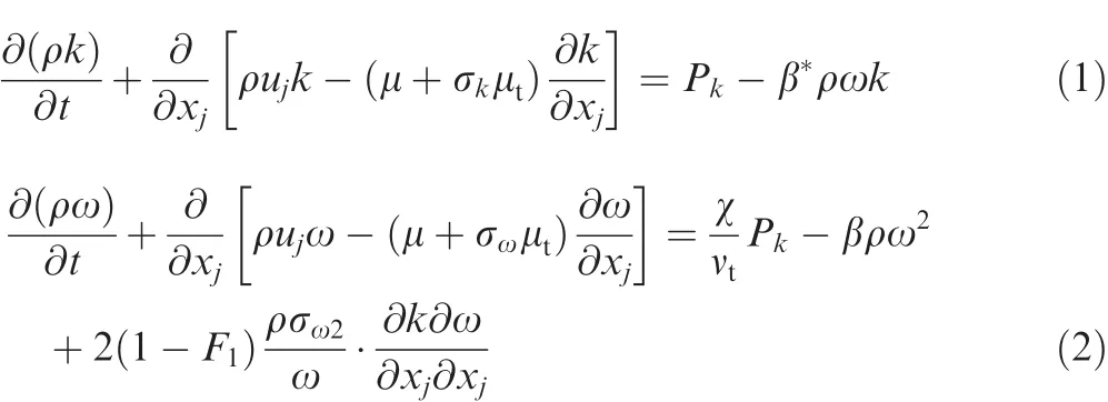
where ρ is density,tis time,kis turbulent kinetic energy,ujis velocity component,xjis coordinate component,ω is speci fic dissipation rate.μ and μtare laminar and turbulent eddy viscosity respectively,νtis kinematic eddy viscosity,β*,β,χ,σk,σω,and σω2are model constants.F1is the blending function and de fined as:

F1=

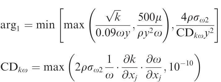
The variableyis the distance from the cell to the nearest wall.Instead of computing the production term exactly,the vorticity magnitude is adopted for approximation:

where the constanta1=0.31,Sis the invariant of strain rate and de fined as:

The blending functionF2is de fined as

Coef ficients of the model are calculated from the formula

The subscript‘1” is for thek- ω model and subscript‘2”is for thek-ε model.Two sets of coef ficients used at present are: σk1=0.85, σω1=0.50, β1=0.075, χ1=5/9, σk2=1.0,σω2=0.856,β2=0.0828,χ2=0.44.

2.2.Description of γ-Reθt and simpli fied transition model

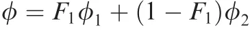
The γ-Reθttransition model is a local correlation-based model,in which the localization is achieved by the de finition of a vorticity Reynolds number and the formulation of a transport equation for transition momentum thickness Reynolds number.Moreover,the intermittency factor is used for the control of production of turbulent kinetic energy.The transport equation for intermittency factor is listed as

where γ is the intermittency factor.

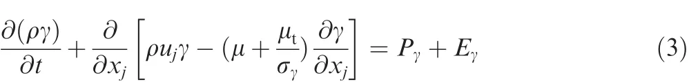
The production and destruction terms of intermittency factor are

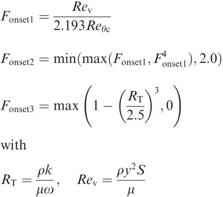
whereFlengthis the transition length function,Fonsetcontrols the onset of transition and de fined as:

Fonset=max（Fonset2-Fonset3，0）

The transport equations for transition momentum thickness Reynolds number is formulated as

whereUis the magnitude of velocity.

The transition Reynolds number in the source term is computed from freestream turbulence intensity and local pressure gradient parameter:

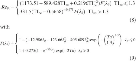
where TI∞is the freestream turbulence intensity and λθis the pressure gradient parameter,they are calculated by

Correlations for critical Reynolds number and transition length function in the original γ-Reθttransition model are

whereReθcis the critical Reynolds number andFlengthis the length function.

The combination of SST turbulence model and γ-Reθttransition model is achieved by multiplying the effective intermittency factor to the production and destruction terms of the turbulent kinetic energy equation,shown as follows:

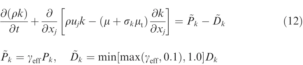
wherePkandDkare the production and destruction terms of the original SST turbulence model.Specially,a correction is proposed for separation-induced transition:the effective intermittency factor is de fined as γeff=max（γ，γsep）.Model coef ficients areca1=2.0,ca2=0.06,ce1=1.0,ce2=50.0,cθt=0.03,σγ=1.0 and σθt=2.0.

The transport equation of transition momentum thickness Reynolds number plays the role of diffusing the freestream value into the boundary-layer.The work of Coder and Maughmer21indicated that the transport equation can be eliminated if a locally-de fined pressure gradient parameter is available.They proposed the parameterHc=yΩ/Uto form the correlations forand showed reasonable results.Actually,the transition momentum thickness Reynolds number is used to calculate the critical Reynolds numberReθcand transition length functionFlength,as shown in Eqs.(10)and(11).If proper correlations forReθcandFlengthcan be supplied,the transport equation can also be removed.According to Ge,23we propose a correlation for the critical Reynolds number using the parameterTwand freestream turbulence intensity:

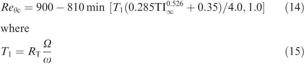
TheT1parameter behaves,to some extent,similarly to theHcparameter,due to the existence of the magnitude of vorticity.The critical Reynolds number decreases with the increase ofT1and has a value between 90 and 900.The transition length function controls the length of transition region and has some effect on the transition onset location.Previous research24indicated that it is appropriate to formulate the function only by the freestream turbulence intensity and a value between 0.1 and 100 is suitable for the function.This leads to the new transition length function as

All of the constants in the correlations in Eqs.(14)and(16)are empirically determined by numerical calculations based on the transitional flat plate.It is noteworthy that the abandon of~Reθtmay result in the inability of prediction for separationinduced transition,as shown in Eq.(13).Although cases with separation are conducted in this paper,no special treatment at present has been made for separation correction,which will be studied in the succeeding work.In addition,the transport equationforintermittencyfactorandtheconnectionwithSSTturbulence model are identical to the original γ-Reθtmodel.

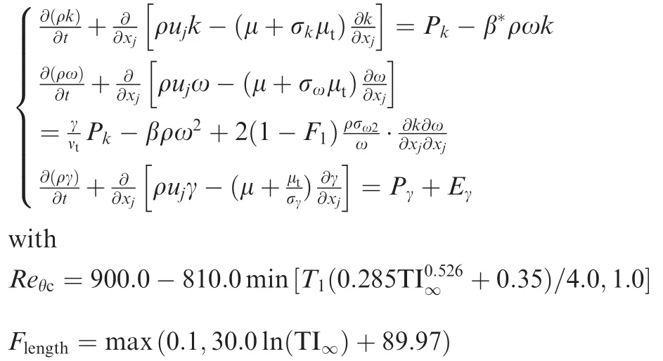
For clear and complete acquaintance of the model,the governing equations and empirical correlations for the simpli fied transition model are summarized as

3.Computational method

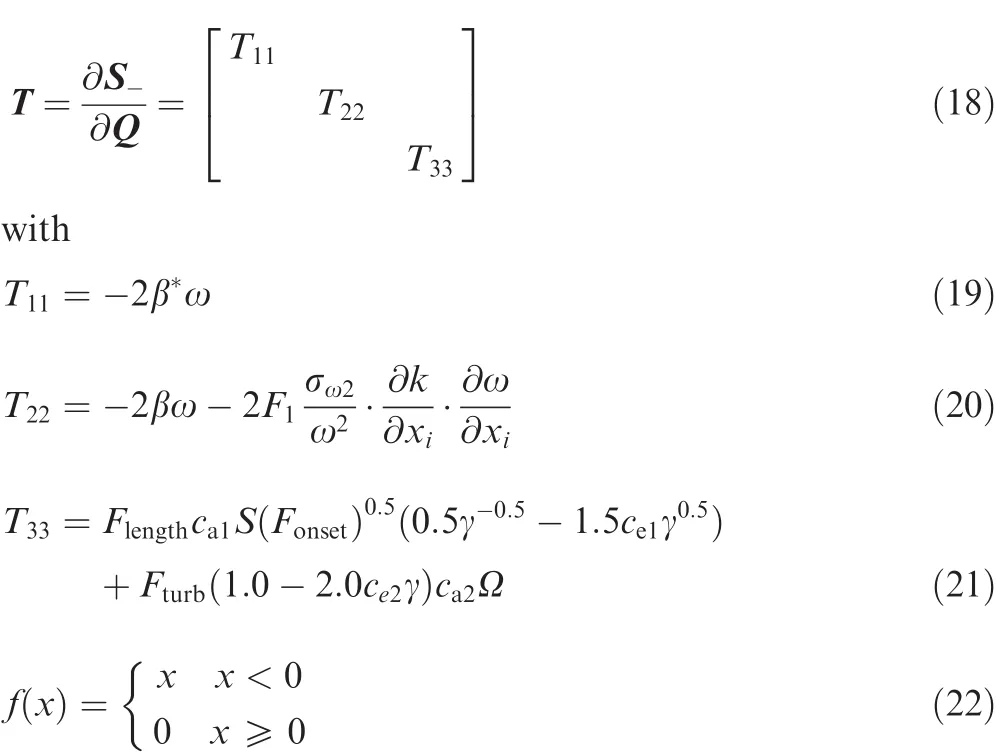
Thenewtransitionmodelinthisworkisimplementedintoaninhouse CFD solver,which is based on finite-volume method and uses multi-block structured grid for simulations.The solver,which is parallelized by massage passing interface(MPI),provides Euler,Navier–Stokes,RANS and even Burnett equations forbothperfectgasandchemicalreactinggas.Inthispaper,only the RANS equations and perfect gas assumption are used for calculations.Concretely,the advection upstream splitting method by pressure-based weight functions(AUSMPW+)25is used to calculate the inviscid fluxes and the viscid fluxes are centrally discretized.The monotone upstream centered scheme for conservationlaws(MUSCL),alongwith thevanAlbada limiter function is adopted for achievement of second-order accuracy.Notably,the turbulence model and transition model equations arealsosolvedbythesecond-orderschemefortheconsideration ofhigh-resolution.Steady-statesolutionsare finallyobtainedby a fully coupled implicit lower–upper symmetric Gauss–Seidel(LU-SGS)26time-marching method,which solves all governing equations simultaneously at each iteration step.Additionally,the source terms of turbulence model and transition model are implicitly treated for the diminution of stiffness problem.Precisely,the negative part of the source terms can be written as:

where S-is the source term and Q the conservative variables.The Jacobian matrix of source term is de fined as

The boundary conditions for turbulent kinetic energy and speci fic dissipation rate at inlet arek∞=1.5（TI∞/100U∞）2and ω∞= ρ∞k∞/μt∞,while their values on the wall arek=0 and ω =60μl/ρβ1y2respectively.The freestream values for γ and~Reθtare given as 1 and 0.0001 respectively,and both of them have a zero flux(∂γ/∂n=0)on the wall.Besides,all freestream conditions are set as the initial conditions for the whole computational domain.

4.Results and discussion

4.1.Zero pressure gradient flat plate

The commonly used Schubauer and Klebanoff case27is a zero pressure gradient flat plate with a Mach number of 0.15.It is a standard test case for the evaluation of performance of new transition models in natural transition.The freestream velocity is 50.1 m/s,freestream turbulence intensity is 0.18%,and unit Reynolds number is 3.4×106.Final results of skin friction coef ficient along the flat plate from three sets of grid and experimental data are shown in Fig.1.Dimensions for Grid 1 to Grid 3 are 154×50,194×90 and 234×130 respectively.All grids are clustered near the solid wall,and the spacing of the first grid to the wall is 1×10-6m,which corresponds to ay-plus value of about 0.15.Similarly,they-plus values for all the following cases are guaranteed to be less than one.We can see from Fig.1 that grid convergence is obtained,since the transition location changes little with the re finement of grid.The present new transition model predicts the transition location,skin friction values in laminar part and in turbulent part accurately except the transition length.The de ficiency of transition length may largely relate to the empirical correlation shown in Eq.(16).In general,the transition model performs much better than the fully laminar and fully turbulent results,especially in the latter part of the flat plate,where the turbulence model under-estimates the skin friction with a value of about 20%.

4.2.Aerospatial-A airfoil

Fig.1 Skin friction coef ficient distribution along Schubauer and Klebanoff flat plate for different grids.

The Aerospatiale-A airfoil,shown in Fig.2,is another typical test case for transition models.The experimental results obtained from ONERA F1 wind tunnel at 13.1°angle of attack are used in this work.28Simulations are carried out at Mach number 0.15,Reynolds number 2.1×106and freestream turbulence intensity 0.2%.Experiment turns out that a laminar separation bubble forms at 12%of the suction side of the chord,resulting in a turbulent boundary-layer downstream.Details of the flow field can be witnessed from the Mach number contour in Fig.3(a),and the separationinduced transition can be clearly seen from Fig.3(b),in which the intermittency factor γ develops rapidly when turbulence occurs.Speci fically,separation occurs at about 80%of the chord and intermittency factor increases signi ficantly when transition occurs.The computed skin friction coef ficientCfalong the suction side of the airfoil is shown in Fig.4(a).We can see that boundary layer transition is accurately predicted from the sharp increase of skin friction obtained by transition models,and good agreement with experimental data is obtained by both the original γ-Reθtand new transition models.The fully turbulent calculation,however,fails to capture the transition onset feature.Fig.4(b)shows the pressure coefficientCparound the airfoil.We can see that the transition models outperform the fully turbulence model signi ficantly except in the trailing edge.The under-prediction of pressure near the trailing edge region can be attributed to the inability of the transition model for simulation of strong flow separation,which occurs at about 83%of the chord as observed in experiment.A closer look at the figure shows that the presented new transition model performs a bit better for the skin friction and the pressure coef ficient in the trailing edge than the original model.Nevertheless,the difference between the two transition models is slight in this case.

4.3.S809 airfoil

The S809 airfoil,designed by the National Renewable Energy Laboratory(NREL),is a primary airfoil used for wind turbine applications.Detailed experimental data,including liftL,dragDand transition locations for different angles of attack α can be found from Somers.29The computational grid is shown in Fig.5,and simulations are performed at Mach number 0.1,Reynolds number 2.0×106and freestream turbulence intensity 0.2%.Fig.6 shows the transition locationsx/con the pressure side and suction side of the airfoil.Speci fically,the transition location on the pressure side moves downstream steadily from about 50%to 60%of the chord as the angle of attack increases,while the transition location on the suction side moves forward sharply at approximate 5°angle of attack due to the adverse pressure gradient.Computed lift coef ficientCLand drag coef ficientCDare depicted in Fig.7,in which we can see that the transition models show apparent improvement for both of the coef ficients,especially for the drag.As expected,transition models possess no distinct advantage over turbulence model at high angles of attack,due to the strong separation.On the whole,good agreement with experimental data is achieved by transition models,and the simpli fied model seems to perform better than the original model.

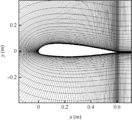
Fig.2 Computational grid for Aerospatial-A airfoil.

Fig.3 Contours of Mach number and intermittency factor for the Aerospatial-A airfoil.

4.4.Hypersonic flat plate

The test case considered for validation of the new transition model in high speed flow is from Mee.30Experiments were carried out in the T4 free-piston shock tunnel at University of Queensland for a 1.5 m long and 0.12 m wide flat plate.Frauholz et al.31studied the case extensively based on the γ-Reθttransition model with modi fied correlations,and satisfactory results were obtained.The freestream conditions for computation are listed in Table 1.The Stanton number is de fined as

where ρ∞,U∞andT0，∞are the freestream density,velocity and total temperature respectively,qwandTware the heat flux and temperature on the wall.It should be noted that the Stanton number measured in experiment has an uncertainty of±18%,as estimated by Mee.30Since the real freestream turbulence intensity in the wind tunnel is unknown,preliminary simulations are performed to tune the transition location,as shown in Fig.8,where TI∞represents the freestream turbulence intensity,and the increase of TI∞promotes the transition of boundary layer.We can also find that the transition location and transition length are strongly affected by the freestream turbulence intensity.The four computed conditions are summarized in Fig.9,and signi ficant improvement of prediction accuracy has been achieved by the transition models,together with the results obtained by Frauholz et al.,31in which the authorspredicted the transitionsby using a modi fied γ-Reθtmodel.Good agreement with experimental data can be witnessed clearly,and it is not an easy task to judge between the two transition models at present.A notable improvement should be mentioned that the new transition model not only predicts the transition onset accurately,but also gets closer to experimental data than the turbulence model on the fully turbulent part of the flat plate.

Fig.4 Skin friction and pressure coef ficients distribution along the Aerospatial-A airfoil.

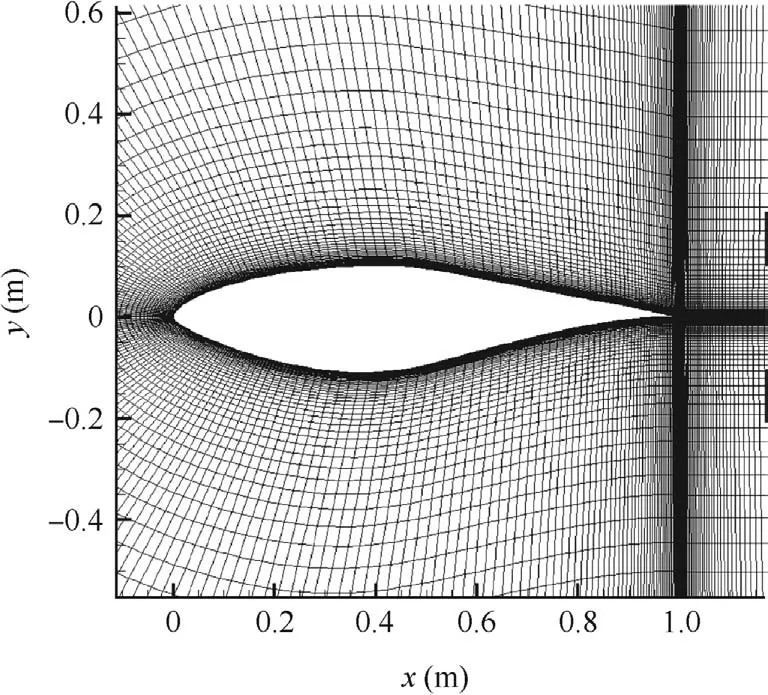
Fig.5 Computational grid for S809 airfoil.

Fig.6 Transition location for S809 airfoil.

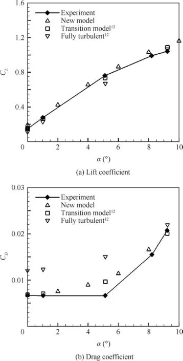
Fig.7 Lift and drag coef ficients at different angles of attack for S809 airfoil.

Table 1 Freestream parameters under different conditions.

4.5.Hypersonic double wedge

A more complicated case for the transition model is the hypersonic double wedge,tested by Neuenhahn and Olivier in the TH2 shock tunnel.32The shape considered at present has a slightly blunted leading edge of 0.5 mm.The first ramp is 178 mm long and has an angle of 9°,while the second ramp is 200 mm long and has an angle of 20.5°.Two-dimensional flow is guaranteed with a width of 270 mm for the geometry.The freestream flow conditions are listed in Table 2 and computational grid is shown in Fig.10.Unlike the previous cases,the hypersonic double wedge encounters severe shock wave/boundary-layer interaction,which can be demonstrated by the Mach number contour obtained by the new transition model in Fig.11.Details of the flow can be noted that a detached bow shock from the blunted leading edge interacts with the separation-induced shock in the corner,followed by a combination with the reattachment shock.

Fig.8 Stanton number distribution of hypersonic flat plate under Condition 1.

Fig.9 Stanton number distribution of hypersonic flat plate under different conditions.

Results of pressure coef ficient and Stanton number are shown in Fig.12.We can see that generally good agreement,especially of the pressure coef ficient,is obtained by the transition model.The fully laminar simulation under-estimates the Stanton number signi ficantly,and has a slightly larger separation zone.On the contrary,the fully turbulent calculation over-estimates the Stanton number and has no separation at all.For comparison,the Stanton number predicted by the original γ-Reθttransition model is extracted from You14and shown in Fig.12(b).We can see that results of the new transition model outperform that of the fully laminar and turbulent assumptions.Speci fically,the new simpli fied model has a relatively lower value of Stanton number and bigger separation zone as compared with the original model.However,discrepancies with experiment still exist for both of the transition models.The absence or inappropriate correction in the transition model for separation flow may be one possible explanation,since the research of You14demonstrated that a more physical meaningful effective intermittency involved pressure gradient performed better.Moreover,some of our previousnumerical attempts indicated that the transition length function and critical Reynolds number correlations have nonnegligible effects on the flow features of transition.Anyway,these aspects are of great importance and will be the key points of the further work.

Table 2 Freestream parameters for hypersonic double wedge.

Fig.10 Computational grid for double wedge.

Fig.11 Contour of Mach number for double wedge.

Fig.12 Pressure coef ficient and Stanton number distribution along double wedge.

5.Conclusions

(1)A simpli fied local-correlation-based transition model has been developed by the removal of the momentum thickness Reynolds number equation in the origin γ-Reθttransition model,along with the new transition length function and critical Reynolds number correlation.

(2)The new transition model is implemented into an inhouse CFD solver and tested for some typical cases,ranging from low speed flows to hypersonic flows.Results from simulations in this work show that the accuracies of the flows are signi ficantly improved by the proposed transition model,compared with the fully laminar and fully turbulent calculations.

(3)It is shown that the simpli fied transition model is comparable to the original γ-Reθtmodel for the simulations presented in this work.The new model appears to be promising and deserves further research due to its satisfactory results and less computational cost than the original model.

(4)It is,however,necessary to validate the new model with more complex test cases for the veri fication of its practicability.Future attempts will be made to the separationinduced transition correction.Besides,the correlations in the model need to be calibrated in detail by wind tunnel data.

Acknowledgement

This study was supported by the State Key Development Program for Basic Research of China(No.2014CB340201).

1.Lee CB.Possible universal transitional scenario in a flat plate boundary layer:measurement and visualization.Phys Rev E2000;62(3):3659–70.

2.Lee CB,Wu JZ.Transition in wall-bounded flows.Appl Mech Rev2008;61(3):30802.

3.Abu-Ghannam BJ,Shaw R.Natural transition of boundary layers–the effects of turbulence,pressure gradient,and flow history.J Mech Eng Sci1980;22(5):213–28.

4.Kalitzin G,Wu X,Durbin PA.DNS of fully turbulent flow in a LPT passage.Int J Heat Fluid Flow2003;24(4):636–44.

5.Yang Z,Voke PR.Large-eddy simulation of boundary-layer separation and transition at a change of surface curvature.J Fluid Mech2001;439:305–33.

6.Michelassi V,Wissink JG,Fr-Ograve J,Rodi W.Large-eddy simulation of flow around low-pressure turbine blade with incoming wakes.AIAA J2003;41(11):2143–56.

7.Yang Z.Large-eddy simulation:past,present and the future.Chin J Aeronaut2015;28(1):11–24.

8.Stock HW,Haase W.Navier-Stokes airfoil computations with eNtransition prediction including transitional flow regions.AIAA J2000;38(11):2059–66.

9.Van Ingen JL.The eNmethod for transition prediction.Reston:AIAA;2008.Report No.:AIAA-2008-3830.

10.Steelant J,Dick E.Modeling of laminar-turbulent transition for high freestream turbulence.J Fluids Eng2001;123(1):22–30.

11.Suzen YB,Huang PG.An intermittency transport equation for modeling flow transition.Reston:AIAA;2000.Report No.:AIAA-2000-0287.

12.Langtry RB,Menter FR.Correlation-based transition modeling for unstructured parallelized computational fluid dynamics codes.AIAA J2009;47(12):2894–906.

13.Walters DK,Leylek JH.A new model for boundary-layer transition using a single-point RANS approachASME 2002 international mechanical engineering congress and exposition.New York:American Society of Mechanical Engineers;2002.

14.You YC,Luedeke H,Eggers T,Hannemann K.Application of the γ-Reθttransition model in high speed flows.Reston:AIAA;2012.Report No.:AIAA-2012-5972.

15.Cheng G,Nichols R,Neroorkar KD,Radhamony PG.Validation and assessment of turbulence transition models.Reston:AIAA;2009.Report No.:AIAA-2009-1141.

16.Malan P,Suluksna K,Juntasaro E.Calibrating the γ-Reθtransition model for commercial CFD.Reston:AIAA;2009.Report No.:AIAA-2009-1142.

17.Kaynak U.Supersonic boundary-layer transition prediction under the effect of compressibility using a correlation-based model.Proc Inst Mech Eng G J Aerosp Eng2012;226(7):722–39.

18.Medida S.Correlation-based transition modeling for external aerodynamic flows[dissertation].Maryland:University of Maryland;2014.

19.Coder JG,Maughmer MD.Computational fluid dynamics compatible transition modeling using an ampli fication factor transport equation.AIAA J2014;52(11):2506–12.

20.Grabe C,Krumbein A.Extension of the γ-Reθtmodel for prediction of cross flow transition.Reston:AIAA;2014.Report No.:AIAA-2014-1269.

21.Coder JG,Maughmer MD.One-equation transition closure for eddy-viscosity turbulence models in CFD.Reston:AIAA;2012.Report No.:AIAA-2012-0672.

22.Menter FR.Two-equation eddy-viscosity turbulence models for engineering applications.AIAA J1994;32(8):1598–605.

23.Ge X.A three-equation bypass transition model based on the intermittency function[dissertation].Ames:Iowa State University;2013.

24.Krause M,Behr M,Ballmann J.Modeling of transition effects in hypersonic intake flows using a correlation-based intermittency model.Reston:AIAA;2008.Report No.:AIAA-2008-2598.

25.Kim KH,Kim C,Rho O.Methods for the accurate computations of hypersonic flows:I.AUSMPW+scheme.J Comput Phys2001;174(1):38–80.

26.Yoon S,Jameson A.Lower-uppersymmetric-Gauss-Seidel method for the Euler and Navier–Stokes equations.AIAA J1988;26(9):1025–6.

27.Schubauer GB,Klebanoff PS.Contributions on the mechanics of boundary-layertransition.Washington,D.C.:NASA;1955.Report No.:NACA TN 3489.

28.Langtry RB.A correlation-based transition model using local variables for unstructured parallelized CFD codes[dissertation].Stuttgart:University of Stuttgart;2006.

29.Somers DM.Design and experimental results for the s809 airfoil.1997.Report No.:NREL/SR-440-6918.

30.Mee DJ.Boundary-layer transition measurements in hypervelocity flows in a shock tunnel.AIAA J2002;40(8):1542–8.

31.Frauholz S,Reinartz BU,Mu¨ller S,Behr M.Transition prediction for scramjet intakes using the γ-Reθtmodel coupled to two turbulence models[Internet].Available from:http://de.arxiv.org/pdf/1410.3946.

32.Neuenhahn T,Olivier H.In fluence of the wall temperature and the entropy layer effects on double wedge shock boundary layer interactions.Reston:AIAA;2006.Report No.:AIAA-2006-8136.