Compressive Sensing for Radar Target Signal Recovery Based on Block Sparse Bayesian Learning

Zhong JinrongWen Gongjian（Science and Technology on Automatic Target Recognition Laboratory， National University of Defense Technology，Changsha 410073， China）

Compressive Sensing for Radar Target Signal Recovery Based on Block Sparse Bayesian Learning

Zhong Jinrong*Wen Gongjian
（Science and Technology on Automatic Target Recognition Laboratory， National University of Defense Technology，Changsha 410073， China）

Nowadays， high-speed sampling and transmission is a foremost challenge of radar system. In order to solve this problem， a compressive sensing approach is proposed for radar target signals in this study. Considering the block sparse structure of signals， the proposed method uses a simple measurement matrix to sample the signals and employ a Block Sparse Bayesian Learning （BSBL） algorithm to recover the signals. The classical BSBL algorithm is applicable to real signal， while radar signals are complex. Therefore， a Complex Block Sparse Bayesian Learning （CBSBL） is extended for the radar target signal reconstruction. Since the existed radar signal compressive sensing models do not take block structures in consideration， the signal reconstruction of proposed approach is more accurate and robust， and the simple measurement matrix leads to an easy implementation of hardware. The effectiveness of the proposed approach is demonstrated by numerical simulations.

Radar signal processing； Compressive Sensing （CS） radar； Block structure； Compressed measurement； Sparse reconstruction

1 Introduction

The higher the resolution of radar， the more details of the target can be captured and more information of the target are available for Automatic Target Recognition （ATR）［1，2］.

Resolution improvement requires additional radar bandwidth. According to the Nyquist theorem， the sampling rate should be twice of thebandwidth. Due to the limited processing speed and data capacity of hardware， a ceiling is set on the sampling rates. Compressive sensing， a new measurement theory proposed by Donoho et al.［3］，indicates that sparse signals can be accurately recovered from lower-rate samplings. Radar signals of targets are sparse， and can be compressively measured and reconstructed［4］.

Compressive measurement and signal reconstruction are two key issues of compressive sensing［5-8］. Most existing compressive sensing approaches employ a random matrix to measure signals. However， the hardware implementation of a random matrix is difficult， which is the largest hindrance in the practice of compressive sensing. Thus， people always pursue an easily realized measurement matrix［9-13］. Radar signals of manmade targets have block structures besides sparsity， which has been not taken into consideration by existed approaches. Researches on speech，electroencephalogram and some other signals［14-22］have demonstrated the block structure is beneficial to the signal reconstruction.

In this paper， an approach of compressive sensing is presented with the block sparse structure of radar target signals both in the compressive measurement and the signal reconstruction steps. In the reconstruction step， it uses a reconstruction algorithm named Complex Block Sparse Bayesian Learning （CBSBL）， which is extended in Ref. ［23］ from the classical BSBL［18，19］， to generate a better reconstruction. Based on the excellent reconstruction algorithm， it is able to use a simple measurement matrix in the compressive sensing. There is only one non-zero element in every row and column of such a measurement matrix. Compared with the traditional compressive sensing approaches， the reconstruction accuracy of our approach is better and the hardware of the measurement matrix is easier to implement. Finally， experiment results exhibit the effectiveness of our compressive sensing model.

2 Compressive Sensing

Suppose the original radar target signal

3 Compressive Sensing for Radar Target Signals

Classical compressive sensing models suppose is just a sparse vector. In applications， it always has certain additional structure such as the block sparse structure［14-16］. With such a structure， vector can be viewed as consisting of non-overlapping blocks， and only a few blocks among them are non-zero.

where， diis the length of block i.

Fig. 1 is a block diagram of the compressive sensing for radar target signals. It consists of two part， the compressive measurement and the signal reconstruction. In the diagram， sR（t） is the original signal， X（fm） is the signal sampled by traditional radars， x is its vector form. We can get， a High Resolution Range Profile （HRRP） of the target， by correlating x with that same pulse in a matched filter （effecting pulse compression）. If we want to generate a high resolution signal，the Analog-to-Digital （A/D） converter requires a high sampling frequency and a large dynamic range. In a compressive sensing radar， a measurements of the original signal is obtained through a compressed measurement matrix Φ， which can be a low-rate A/D converter. From the measureddata y， we can get a reconstruction of the original signal sR（t）， or reconstructions of the digital signal x and， from y. Since sR（t） is analog and not convenient to discuss， we take the wanted high-rate sampled signal X（fm） as the original signal in the following discussion. In our compressive sensing model， we reconstruct the sparse vector of target，， from the compressive measurements y， and then recover the frequency-domain signal byFinally， the HRRP of target is generated by an Inverse Fast Fourier Transform （IFFT）， which effect matched filter and pulse compression.

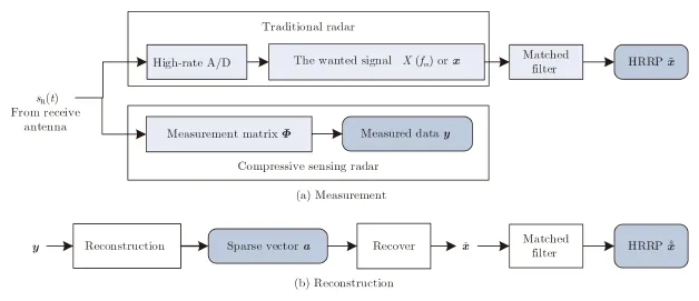
Fig. 1 Compressive sensing for radar target signals

In Subsection 3.1， the block structure of radar target signals and the sparse representation of the signals are discussed briefly. In Subsection 3.2， a simple matrix is suggested for compressive measurement. In Subsection 3.3， the method of signal reconstruction from compressive samples is discussed.

3.1Sparsity and block structure of radar target signals

Fig. 2 shows a radar target signal in the frequency domain and time domain （only amplitude）. The time domain signal can also be referred to as HRRP.

The original radar target signal in frequency domain is X（fm） or in vector form x， while the complex time domain signal is denoted as. In the application of radar ATR system based on HRRP of targets， the observation ranges of radars are far larger than the size of a target. The scattering centers of some targets， such as airplanes and missiles， are sparse and located on a few blocks ofIn other words，has a with block structure. Moreover， there may be intra-block correlation［18，19］. In the high-frequency region， radar targets can be represented by a few scattering centers， then radar target signals can be sparsely represented by the echoes of these scattering centers［26，27］.

Fig. 2 HRRP of a target， the below one is HRRP， the above one is its frequency-domain transform

Here， rpis the position of scattering center p. fmis the frequency of samplings. V（fm） is noise. and Ep（fm；rp） is the response of scattering center p. The isotropic point scattering model is given by Ep（fm；rp）=exp（-j4πfmrp/c）. Here， c is the speed of light. There is sparsity in x， as the scattering centers of radar targets are sparse in space. Base on it， we construct the dictionary for radar sig-nals of targets. Suppose that the unambiguous distance of radar is R. The start point is r0. We sample the unambiguous distance into N points with spacing ΔR. For every position rn=r0+nΔR，

Ψnis an atom of dictionary and φm，nis an element of the atomic. The signal x is sparse on the dictionary Ψ. The radar signals of targets can be represented Eq. （1）， x=Ψ.a. Here， a is a sparse representation vector of x. The number of dictionary column， as well as the length of the sparse vector， is N. As the time domain signal have block structures， a is also a block sparse vector based on such a dictionary. It may be with intrablock correlation［18，19］.

3.2Measurement matrix

Most existing compressive sensing models take a random matrix Φ*， as shown in Fig. 3（a），as the measurement matrix. In our compressive model， we use a simple measurement matrix Φ， as shown in Fig. 3（b）. There is only one non-zero element in each row or each column of matrix Φ. Actually， the measurement matrix shown in Fig. 3 is equivalent to an unequally-space sampling method. It not only reduces size of samplings， but also can relieve the pressure of A/D conversion.

The unequally down-sampling in the frequency domain can retain more information，though aliasing arises in the time domain. Since the signal is block sparse and most of the areas are zero， the aliasing can be suppressed by a

~ sophisticated reconstruction algorithm. Therefore，it is reasonable to take Φ as a measurement matrix. The compressive measurement is given by，

Here， v is a noise vector. The sensing matrix is Θ=Φ.Ψ. Actually， in our compressive sensing model， as the measurement matrix Φ is known，we can construct the sensing matrix Θ directly， Here， the atom isAnd every element is given by θq，n=exp（-j4πfqrn/c）. fqis the frequency of q-th sampling. Q is the number of samplings.

3.3CBSBL signal reconstruction algorithm

Recovering a from compressive measurement data is an important procedure of compressive sensing. Recently， an excellent recover algorithm named BSBL algorithm is proposed by Zhang and Rao［13，15］. It has a superior ability to recover block sparse signals. Compared to Group Lasso［16］， Mix-L1/L2［28］， and Block-OMP［29］， DSG［30］， CluSSMCMC［31］， SD-SPR［32］etc.， BSBL algorithm does not need any prior knowledge of blocks. Moreover， BSBL algorithm can exploit the intrablock correlation. As the distribution of block structures of radar target signals is unknown， BSBL algorithm is preferred for radar target signal reconstruction.

Fig. 3 Two different measurement matrices

The BSBL algorithm is proposed for real signals， but radar signals are complex. It is not directly applicable to radar signals. Dr. Zhang gives a solution， in which we have to decompose the complex signal and sensing matrix into a real part and an imaginary part first. Then we can obtain a real signal model as Eq. （8）. We name it as Bin-ary-channels-BSBL （Bi-BSBL） algorithm.

In order to recover complex signals directly，we extend the advanced BSBL framework into the complex domain， and then present the EM-iteration algorithm［19］in the CBSBL framework.

and （12） are the complex-domain-extended block sparse Bayesian learning framework. The learning lure of these parameters is the key issue of the Bayesian learning method. There are many different solution algorithms according to iterative methods of Eqs. （11） and （12）. Two iteration methods， EM-iteration and BO-iterative are presented in Refs. ［18，19］ for real signals. We extend the EM iteration algorithm to complex signals. Based on the estimation theory of complex statistical signal processing and complex signals Bayesian method［33］， we outline the iterative formulae as follows.

Iteration：

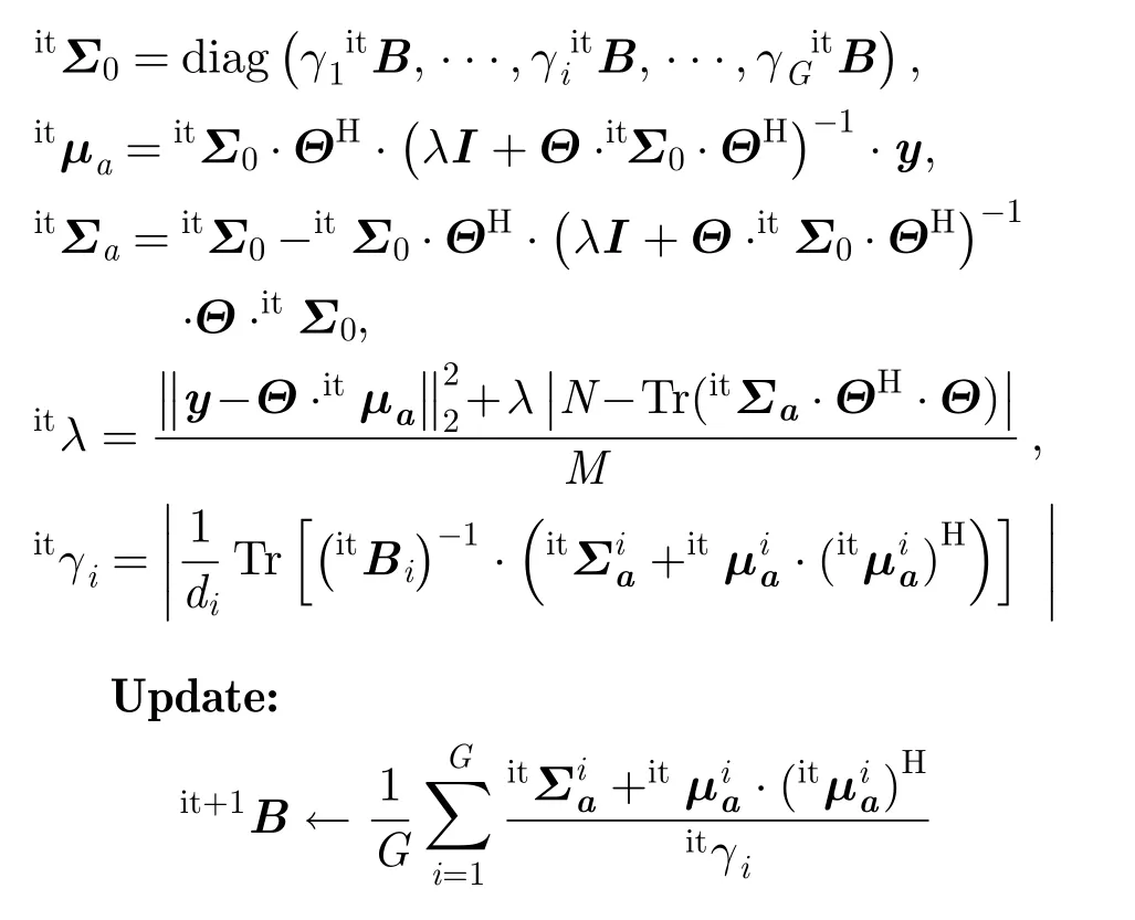
If γi≤δγ， set Bi=0. In order to prevent a problem with over-fitting， it is assumed that the structure of each block is the same， i.e.The iteration termination criterion is：

or the maximum number of iterations Nδis reached. Suppose the index of stop iteration is nδ.

It is necessary to point out that the CBSBL algorithm is not a novel algorithm， but the complex extension of the BSBL algorithm. It inherits the capability of exploiting block structure and intra-block correlation.

4 Experimental Results

First， the performance of our CBSBL reconstruction algorithms is examined， in comparing with Bi-BSBL， Orthogonal Matching Pursuit（OMP）， and SBL algorithms. The last two algorithms do not exploit block structure， while the Bi-BSBL does. Second， we analyze the reconstruction accuracy when the original signals are meas-ured by the simple measurement matrix Φ， in construction with the results of experience in which the signals are measured by the random matrix Φ*.

Experimental data is recoded in microwavedarkroom. The radar emits a step-frequency signal， with start frequency fs=8.5 GHz， stop frequency fe=9.5 GHz， and bandwidth B = 1 GHz. The resolution is dR=0.15 m， and radar un-aliasing distance is R=15 m. We set the spacing ΔR=0.15 m to sample the distance R. The length of vector α is N=101. We add Gaussian white noise and make signal-to-noise ratio SNR=20 dB. In this paper， SNR is defined as SNR=are the energy of signal and noise respectively. ρ is the compressive measurement ratio. The number of samplings at every compressive measurement ratio is M=sup（ρN）. ρ is set to 10 values in range［0.25，0.7］， with the interval Δρ=0.05. Experiments were repeated Tn=50 times at each ρvalue. Noise v and observation matrix Φ are regenerated every iteration. The Mean Square Error （MSE） of every algorithm is given by

4.1Experiment exploiting block structure in reconstruction

In this subsection， the measurement matrix is a random matrix Φ*. Then， we test the reconstruction accuracy of the four algorithms. The sparse parameter of OMP is set as K=25 which is a parameter chosen by prior knowledge of the target. SBL， Bi-BSBL， CBSBL iterate 1000 times separately. Fig. 4 shows MSEs of four algorithms.

It can be found from Fig. 4（a） that the reconstruction accuracy of CBSBL algorithm is better than the OMP and SBL algorithms. Fig. 4（b）shows that the reconstruction accuracy of CBSBL algorithm is almost the same as the Bi-BSBL algorithm. When the compressive ratio is low， the performance of CBSBL is a little better than the Bi-BSBL. This demonstrates CBSBL and Bi-BSBL，the algorithms exploiting block structure， obtain better signal reconstructions than those that do not.

For a straightforward observation， Fig. 5 shows the reconstructed HRRPs of the four algorithms in an experiment trip. Figs. 5（a）～5（d）are the reconstructions of CBSBL algorithm， Bi-BSBL algorithm， SBL algorithm， and OMP algorithms respectively. The reconstructed HRRPs in Figs. 5（a） and 5（b） are more similar to the original signal， while the reconstructed results of SBL and OMP algorithms have obvious waveform distortion. Clearly， the signals are recovered better by CBSBL and Bi-BSBL.

4.2Experiment exploiting block structure with simplemeasurement matrix

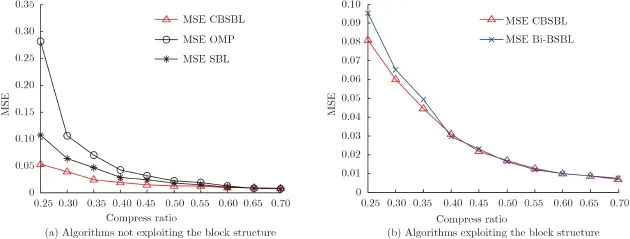
Fig. 4 Reconstruction MSEs of different algorithms， when the sampling matrix is Φ*

In this subsection， we use a simple measurement matrix Φ to measure the original signals，and then use CBSBL， Bi-SBSL， SBL， OMP algorithms to recover the signals. The experimentalsetting of this section is the same as for Subsection 4.1.

Fig. 6 shows the reconstruction accuracy of the four algorithms. Comparing with the results in Fig. 4， we can find that the reconstruction MESs are almost the same. Only slight degradations have appeared. Figs. 7（a）～7（d） show the reconstructions of the four algorithms in one time experiment.The same conclusion， the signals CBSBL and Bi-BSBL algorithms reconstruct signals better， can be drawn from the reconstruction results in Fig. 7.

4.3Reconstruction accuracy under different noise levels

Fig. 5 Reconstructed HRRPs of different algorithms in one trip， when the sampling matrix is Φ*and ρ=0.4

Fig. 6 Reconstruction MSEs of different algorithms， when the sampling matrix is Φ

In this subsection， we set ρ=0.35， and add Gaussian white noise to the original signals to let SNR=［15，20，25，30，35，40］ dB. Then the number of compressive samplings is M=sup（0.35×101）=36. For each fixed SNR， we carry out the compressive measure and reconstruction for Tn=50 trips. The reconstruction MSEs of CBSBL and Bi-BSBL versus SNR are shown in Fig. 8. It can be seen that the reconstruction accuracy of the CBSBLalgorithm is a little better than Bi-BSBL under different noise levels.

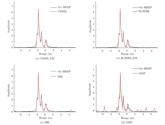
Fig. 7 Reconstructed HRRPs of different algorithms in one trip， when the sampling matrix is Φ*and ρ=0.4

Fig. 8 Reconstruction MSEs and time cost

4.4Time efficiency of CBSBL and Bi-BSBL

The recover accuracy of the CBSBL algorithm has been investigated in Subsections 4.1，4.2， and 4.3. In this subsection， we present the time efficiency. Because accuracy is the primary goal in signal reconstruction， we only compare the efficiency of CBSBL algorithm and Bi-BSBL algorithm， but not OMP and SBL. We use the CPU time as measure of complexity. Although it is not an exact measure， it gives a rough estimation. The comparison is performed in MATLAB2014A environment on a computer with Intel four-core 3.4 GHz CPU and 4.0 Gb RAM，and windows 7 OS.

Fig. 9 Consumed time versus compressive ratios

Fig. 9 shows the consumed time of reconstruction versus compression ratios， ρ. Here， we set the SNR as SNR=20 dB. It can be seen that the CBSBL algorithm uses less time than Bi-BSBLunder different compressive ratio levels. Fig. 10 shows the reconstruction cost time versus SNRs.Here， the compressed ratio is ρ=0.35. It is shown that the CBSBL algorithm is less time-intensive than Bi-BSBL under different noise levels.

Fig. 10 Consumed time versus SNRs

5 Conclusions

In this study， we first extend a CBSBL reconstruction algorithm for complex signals， such as radar signals. Compared to the Bi-BSBL method that decomposes signals into two channels， CBSBL has better reconstruction accuracy and efficiency. Based on the CBSBL signal reconstruction algorithm， we present a compressive sensing model for radar target signals that exploits the block structure of signals. It utilizes a measurement matrix， which is easy to realize in hardware. Experiments demonstrated the effectiveness of our compressive sensing model.

［1］Du L， Wang P， Liu H， et al.. Bayesian spatiotemporal multitask learning for radar HRRP target recognition［J］. IEEE Transactions on Signal Processing， 2011， 59（7）： 3182-3196.

［2］Shi L， Wang P， Liu H， et al.. Radar HRRP statistical recognition with local factor analysis by automatic Bayesian Ying Yang harmony learning［C］. IEEE International Conference on Acoustics Speech and Signal Processing （ICASSP）， Dallas Texas USA， 2010： 1878-1881.

［3］Donoho D L. Compressed sensing［J］. IEEE Transactions on Information Theory， 2006， 52（4）： 1289-1306.

［4］Baraniuk R and Steeghs P. Compressive radar imaging［C］. IEEE Radar Conference， Boston， Apr. 2007： 128-133.

［5］Ender J H G. On compressive sensing applied to radar［J］. Signal Processing， 2010， 90（5）： 1402-1414.

［6］Xie X C and Zhang Y H. High-resolution imaging of moving train by ground-based radar with compressive sensing［J］. Electronics Letters， 2010， 46（7）： 529-531.

［7］Hereman M and Strohmer T. High-resolution radar via compressed sensing［J］. IEEE Transactions on Signal Processing， 2009， 57（6）： 2275-2284.

［8］Patel V M， Easley G R， Healy D M， et al.. Compressed synthetic aperture radar［J］. IEEE Journal of Selected Topics on Signal Processing， 2010， 4（2）： 244-254.

［9］Devore R A. Deterministic construction of compressed sensing matrices［J］. Journal of Complexity， 2013， 23（4）： 918-925.

［10］Ni K and Datta S. Efficient deterministic compressed sensing for images with chirps and reed-muller codes［J］. SIAM Journal on Imaging Sciences， 2011， 4（3）： 931-953.

［11］Li S X， Gao F， Ge G N， et al.. Deterministic construction of compressed sensing matrices via algebraic curves［J］. IEEE Transactions on Information Theory， 2012， 58（8）：5035-5041.

［12］Abolghasemi V， Ferdowsi S， and Sanei S. A gradient-based alternating minimization approach for optimization of the measurement matrix in compressive sensing［J］. Signal Processing， 2012， 92（3）： 999-1009.

［13］Donoho D L and Tsaig Y. Sparse solution of underdetermined systems of linear equations by stage wise orthogonal matching pursuit［J］. IEEE Transactions on Information Theory， 2012， 58（2）： 1094-1121.

［14］Baraniukr， Cevher V， Duarte M， et al.. Model-based compressive sensing［J］. IEEE Transactions on Information Theory， 2010， 56（4）： 1982-2001.

［15］Asaeia， Golbabaee M， Bourlard H， et al.. Structured sparsity models for reverberant speech separation［J］. IEEE Transactions on Audio， Speech， and Language Processing，2014， 22（3）： 620-633.

［16］Yuan M and Liu Y. Model selection and estimation in regression with grouped variables［J］. Journal of the Royal Statistical Society Series B， 2006， 68（1）： 49-67.

［17］Sun H， Zhang Z L， and Yu L. From sparseity to structured sparsity： Bayesian perspective［J］. Signal Processing， 2012，28（6）： 760-773 （in Chinese）.孙洪， 张智林， 余磊. 从稀疏到结构化稀疏： 贝叶斯方法［J］. 信号处理， 2012， 28（6）： 760-773.

［18］Zhang Z L and Rao B D. Recovery of block sparse signals using the framework of block sparse Bayesian learning［C］. IEEE International Conference on Acoustics， Speech and Signal Processing （ICASSP）， Kyoto， Japan， Mar. 2012：3345-3348.

［19］Zhang Z L and Rao B D. Extension of SBL algorithms for the recovery of block sparse signals with intra-block correlation［J］. IEEE Transactions on Signal Processing， 2012，61（8）： 2009-2015.

［20］Babacan S D， Nakajima S， and Do M N. Bayesian groupsparse modeling and variational inference［J］. IEEE Transactions on Signal Processing， 2014， 62（11）： 2906-2921.

［21］Liu B Y， Zhang Z L， Xu G， et al.. Energy efficient telemonitoring of physiological signals via compressed sensing： A fast algorithm and power consumption evaluation［J］. Biomedical Signal Processing and Control， 2014， 11（1）： 80-88.

［22］Shen Y， Duan H， Fang J， et al.. Pattern-coupled sparse bayesian learning for recovery of block-sparse signals［J］. IEEE Transactions on Signal Processing， 2013， 63（2）：1896-1900.

［23］Zhong J R， Wen G J， and Ma C H. Radar signal reconstruction algorithm based on complex block sparse Bayesian learning［C］. 12th International Conference on Signal Processing， Hangzhou， China， Oct. 2014： 1930-1933.

［24］Davies M E and Gribonval R. Restricted isometry constants where lp sparse recovery can fail for 0＜p≤1［J］. IEEE Transactions on Information Theory， 2009， 55（5）：2203-2214.

［25］Wipf D P and Rao B D. Sparse Bayesian learning for basis selection［J］. IEEE Transactions on Signal Processing， 2004，52（8）： 2153-2164.

［26］Potter L C and Moses R L. Attributed scattering centers for SAR ATR［J］. IEEE Transactions on Image Processing，1997， 6（1）： 79-91.

［27］Potter L C， Chiang D M， Carriere R， el al.. A GTD-based parametric model for radar scattering［J］. IEEE Transactions on Antennas and Propagation， 1995， 43（10）：1058-1066.

［28］Eldar Y C， Kuppinger P， and Bolcskei H. Block-sparse signals： uncertainty relations and efficient recovery［J］. IEEE Transactions on Signal Processing， 2010， 58（6）： 3042-3054.

［29］Eldar Y C and Mishali M. Robust recovery of signals from a structured union of subspaces［J］. IEEE Transactions on Information Theory， 2009， 55（11）： 5302-5316.

［30］Huang J Z and Zhang T. METAXAS D. Learning with dynamic structured sparsity［J］. Journal of Machine Learning Research， 2012， 12（7）： 3371-3412.

［31］Yu L， Sun H， Barbot J P， et al.. Bayesian compressive sensing for cluster structured sparse signals［J］. Signal Processing， 2012， 92（1）： 259-269.

［32］Peleg T， Eldar Y and Elad M. Exploiting statistical dependencies in sparse representations for signalrecovery［J］. IEEE Transactions on Signal Processing， 2012， 60（5）： 2286-2303.

［33］Steven M. K. Fundamentals of Statistical Signal Processing Volume I： Estimation Theory［M］. Englewood Cliffs， NJ，USA， Prentice Hall， IInc.， 1993： 493-567.罗鹏飞， 张文明等译. 统计信号处理基础--估计与检测理论［M］.北京： 电子工业出版社， 2006： 397-440.

Zhong Jinrong was born in Guangxi，China in 1985. He received the BS and MS degrees from National University of Defense Technology in 2008， and 2010， respectively. He is a doctoral candidate in information and communication engineering at the Key Laboratory of ATR， National University of Defense Technology. His main interests are automatic target recognition， radar target characteristics， and radar signal processing.

E-mail： zhong_nudt@163.com

Wen Gongjian was born in Changsha，China in 1972. He received the BS，MS， and Ph.D. degrees from National Universityof Defense Technologyin 1994， 1997， and 2000， respectively. Then he went through two years of postdoctoral work at Wuhan University. He is currently a Professor with National University of Defense Technology and the head of the fourth department of the key laboratory of ATR. He is mainly interested in remote sensing，photogrammetry， and image understanding.

10.12000/JR15056

Reference format： Zhong Jinrong and Wen Gongjian. Compressive sensing for radar target signal recovery based on block sparse Bayesian learning［J］. Journal of Radars， 2016， 5（1）： 99-108. DOI： 10.12000/JR15056.

引用格式：钟金荣， 文贡坚. 基于块稀疏贝叶斯学习的雷达目标压缩感知［J］. 雷达学报， 2016， 5（1）： 99-108. DOI：10.12000/JR15056.

基于块稀疏贝叶斯学习的雷达目标压缩感知

钟金荣 文贡坚

（国防科技大学自动目标识别重点实验室 长沙 410073）

高速采样和传输是目前雷达系统面临的一个重要挑战。针对这一问题，该文提出一种利用信号块结构特性的雷达目标压缩感知方法。该方法采用一个简单的测量矩阵对信号进行采样，然后运用块稀疏贝叶斯学习算法恢复信号。经典的块稀疏贝叶斯学习算法适用于实信号，该文将其扩为可直接处理雷达信号的复数域稀疏贝叶斯算法。相对于现有压缩感知方法，该方法不仅具有更好的信号重构精度和鲁棒性，更重要的是其压缩测量矩阵形式简单、易于硬件实现。数值仿真实验结果验证了该方法的有效性。

雷达信号处理；压缩感知雷达；块结构；压缩测量；稀疏重构

TN957.52

A

2095-283X（2016）01-0099-10

Manuscript received May 11， 2015； revised February 1， 2016. Published online February 2， 2016.

The New Century Excellent Talents Supporting Plan of Ministry Education （No.NCET-11-0866）.

*Communication author： Zhong Jinrong.

E-mail： zhong_nudt@163.com.

CLC index： TN957.52