Ensemble Transform Sensitivity Method for AdaptiveObservations

Yu ZHANG,Yuanfu XIE,HongliWANG,DehuiCHEN,and Zoltan TOTH

1Nanjing University ofInformation Science and Technology,Nanjing 210044

2Chinese Academy ofMeteorological Science,Beijing 100081

3GlobalSystems Division,Earth System Research Laboratory,NOAA,Boulder,CO 80305,USA

4Cooperative Institute forResearch in the Atmosphere,Colorado State University,FortCollins,CO 80523,USA

5NationalMeteorologicalCentre,Beijing 100081

Ensemble Transform Sensitivity Method for AdaptiveObservations

Yu ZHANG1,2,3,Yuanfu XIE3∗,HongliWANG3,4,DehuiCHEN5,and Zoltan TOTH3

1Nanjing University ofInformation Science and Technology,Nanjing 210044

2Chinese Academy ofMeteorological Science,Beijing 100081

3GlobalSystems Division,Earth System Research Laboratory,NOAA,Boulder,CO 80305,USA

4Cooperative Institute forResearch in the Atmosphere,Colorado State University,FortCollins,CO 80523,USA

5NationalMeteorologicalCentre,Beijing 100081

The Ensemble Transform(ET)method has been shown to be useful in providing guidance for adaptive observation deployment.Itpredicts forecasterrorvariance reduction foreach possibledeploymentusing itscorresponding transformation matrix in an ensemble subspace.In this paper,a new ET-based sensitivity(ETS)method,which calculates the gradientof forecast error variance reduction in terms of analysis error variance reduction,is proposed to specify regions for possible adaptiveobservations.ETS isa fi rstorderapproximation of the ET;itrequires justone calculation ofa transformationmatrix, increasing computational efficiency(60%–80%reduction in computational cost).An explicitmathematical formulation of the ETSgradient is derived and described.Both the ET and ETSmethods are applied to the Hurricane Irene(2011)case and a heavy rainfall case for comparison.The numerical results imply that the sensitive areasestimated by the ETSand ET are similar.However,ETS ismuchmore efficient,particularly when the resolution is higher and the number of ensemble members is larger.

adaptive observation,high impactweather,ensemble transform

1. Introduction

For high-impactweather(HIW)events,adaptivemobile observation instruments or vehicles can be deployed to improve analysis quality and forecast accuracy.Several field campaignshave shown thatobservations sampled in dynamically sensitive areas have positive impacts on numerical weather prediction(Majumdar etal.,2001;Majumdar etal., 2011).For example,1–2 day forecastskillwas increased by assimilating targeted datadeployed in the Frontsand Atlantic Storm Track Experimentand the North Pacific Experiments (Joly et al.,1997;Joly et al.,1999;Langland et al.,1999a; Langland et al.,1999b).Assim ilation of adaptive observationssignificantly reduced typhoon track forecasterrorsover the western North Pacific and the Atlantic(Aberson,2003; Wu etal.,2007a;Aberson etal.,2011;Chou etal.,2011).

A major challenge is to identify sensitive areas for deploying theadaptiveobservations in the hoursor daysahead of HIW events.There are severalapproaches thathave been developed to estimate sensitive areas,such as the singular vector method(Palmer et al.,1998;Buizza and Montani, 1999),theconditionalnonlinearoptimalperturbationmethod (Mu et al.,2009;Wang etal.,2011),and the adjoint sensitivity method(Wu et al.,2007b,2009).In general,an adjointmodel isusually required in theabove threeapproaches. In addition,ensemble-basedmethods,such as the ensemble transformation(ET)method(Bishop and Toth,1999),the ensemble transform Kalman fi lter(ETKF)method(Bishop et al.,2001),and ensemble sensitivity(Ancell and Hakim, 2007)arew idely used in field campaigns(Chang etal.,2013; Xieetal.,2013).

The ensemble-based methods are less demanding computationally and have been extensively employed in practical applications(Ancell and Hakim,2007;Ito and Wu,2013). Thesemethods consider sensitivity in the subspace spanned by the ensemble forecasts and are computationally inexpensive in operational centerswhere ensemble forecastsare routinely produced.Among these methods,ET(Bishop and Toth,1999;hereafter BT1999)provides a practicalmethod foradaptive observations.Ithasbeen used for targeted dropsonde deployments in w inter storm reconnaissance(WSR) (Szunyogh et al.,2000).Later,ETKF was used to identify the sensitive region in WSR(Szunyogh et al.,2002).The dropsonde data collected over these sensitive areas improved theweather forecasts over the continental United States andAlaska(Szunyoghetal.,2000).However,the impactofdropsonde datamay be limited in global forecasts(Ham illetal., 2001),and high-resolution observation datasetsaresuggested for HIW(Bauer etal.,2011,Bergeretal.,2011).

It is noted that ET is still expensive for high-resolution applicationsor those applicationsw ith large numbersof ensemblemembers.ET has been used at relatively coarse resolutions and a few vertical levels,e.g.,usually three vertical levels at the National Centers for Environmental Prediction (NCEP),and a relatively small number of ensemblemembers(30–60).As resolutions increase for HIW applications, the computational costgrows exponentially.This is because ET,aswell as the ETKF,has been implemented to exhaust all possible observation deployments.For example,it currently estimates sensitive areas by adding an observation at every analysis grid location,horizontally and vertically,and calculating theensemble transformation and the reduction of forecastvariance foreach observation.Becauseof theuseof amatrix decomposition of ensemble covariance,the computational costalso increasesasa cubic function of the number ofensemblemembers.Forhigh-resolution adaptiveobservation applications,or those w ith large numbers of ensemble members,the computationalcostcould be significant.ETKF can also be computationally expensive,the same as the ET method(Bishop et al.,2001).In order to further improve thesemethods for fine scale HIW applications,efficiency is an important factor to investigate.

A new ET-based sensitivity(ETS)method is proposed in this paper to specify sensitive regions for adaptive observations.The proposedmethod calculates the sensitivity(gradient)of forecasterror variance reduction in terms of analysis error variance reduction.Thenew ly proposed ETSmethod is the fi rstorder approximation of the original perturbation ET method and reducescomputationalcostbecauseonly asingle transformationmatrix calculation is required.

This paper is organized as follows.In section 2,we review the ET method.In section 3,we describe how ETS calculates the sensitivity w ith a single transformationmatrix calculation.We compare sensitive regionsusing ET and ETS for a hurricane case and a heavy rainfall case in section 4. Conclusionsand discussionsarepresented in section 5.

2. Review of the ETmethod

First,we review theETmethod(BT1999),with somematrix notations used to simplify the discussion(see Table 1). This review inmatrix forms helps illustrate the ETS derivation.

2.1. Forecasterrorestimation using a transformationmatrix

Let EEE(t)denote a set of ensemble forecasts at a given forecast time t.This EEE(t)is amatrix w ith Mrows and K columns,where Mis the numberof gridded valuesof all the state variables and K is the number of ensemblemembers. Then,the ensemble perturbationmatrix XXXeisalso an M×K matrix,

Here is theadaptiveobservation strategy in ET:Usea set of ensemble forecasts EEE(t)to determ inewhich possible deploymentsofobservational resourcesata futureanalysis time tfaw illm inim ize theexpected prediction errorof forecasts for the verification time tv,which are initialized w ith,inter alia, thesupplementaldata taken at tfa(BT1999).

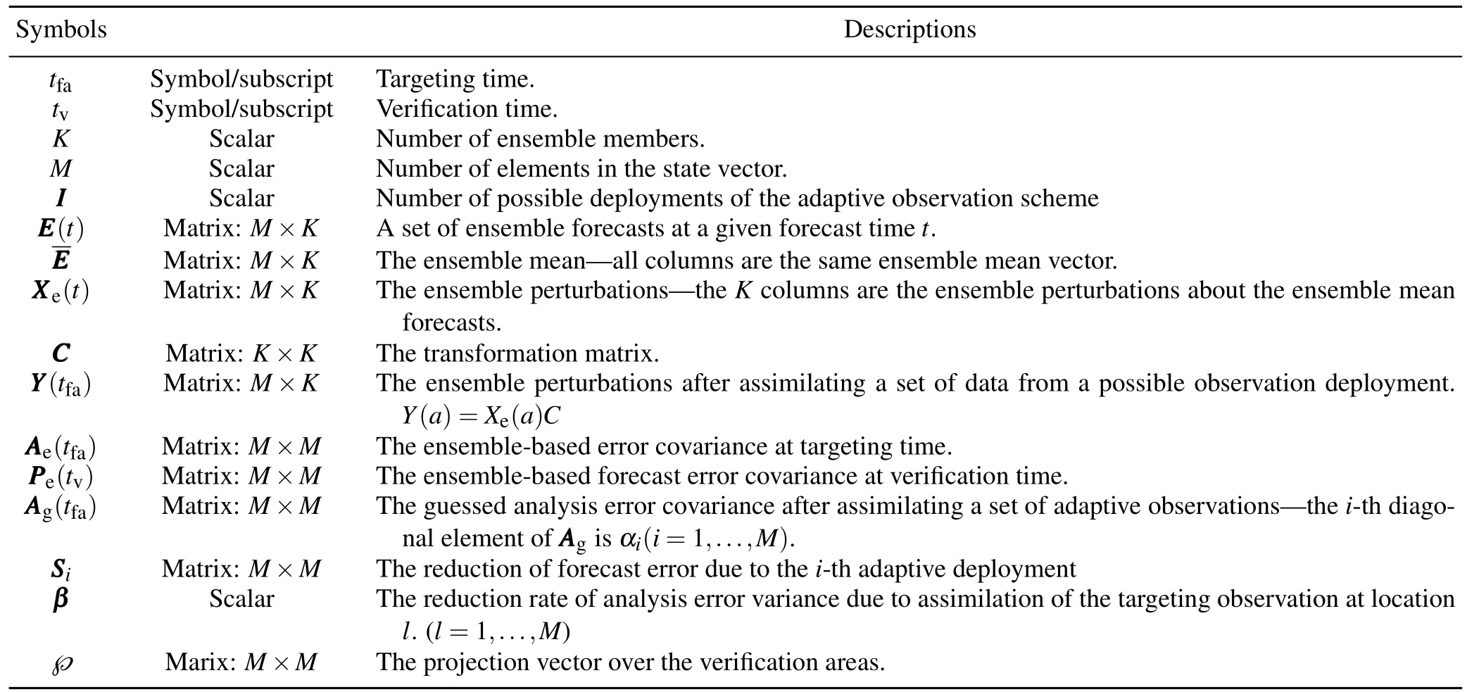
Table 1.Importantsymbols.

Let XXXe(tfa)denote the perturbationsat tfa,XXXe(tv)the perturbationsat the tv,and YYY(tfa)the ensemble perturbationsafter assim ilating a setof data from a possible adaptive obser-vation deployment.ET findsa transformation of the ensemble perturbation XXXe(tfa)to YYY(tfa).Such a transformation can be uniquely determ ined if the number of ensemble forecasts is very large and unconstrained(Anderson,1997).Assume sucha transformationexists,and denote itasamatrix CCC,such that

This CCC isa K×K matrix.

Mathematically,the ensemble-based error covariance at the taapproximates the truth analysis error covariance of AAAe(tfa),

The ensemble-based forecast error covariance at tv,PPPe(tv), can be approximated by

In reality,the true analysis error covariance of AAAe(tfa)is unknown,but an approximation or guess can be estimated by a given data assim ilation system(BT1999).Let AAAg(tfa) denote the approximation of AAAe(tfa)and Eq.(3)is approximately satisfied.Thus,forcing transformed ensemble-based error covariance to be equal to the guessed adaptive analysis error covariance,

The ETmethod finds a solution of CCCCCCTsatisfying Eq.(5). Note that there is really no need to explicitly calculate the transformationmatrix CCC in the ETmethod but CCCCCCT,a productof the transformation.For the sakeof simplicity,herewe assume that AAAgisa full rankmatrix(BT1999)and Eq.(5)can be rew ritten as

Then if XXXe(tfa)isa full rank(e.g.,asetof independentensemblemembers),thematrixisinvertible.By multiplyingand XXXe(tfa)from the leftand rightof Eq. (5′),thesolution of theproductof the ET transformationmatrix(BT1999)is,

Equation(6)is an equivalentvariation of the Equation(8)in BT1999.Thismatrix derivation of the productsimplifies the derivation of BT1999.

2.2. Measurementofadaptive observation sensitivity

Letβbe a parametermeasuring the percentage reductions in the analysiserroraftera setof adaptiveobservations are assim ilated.For example,β=1means zero percent reduction,β=0.5means50%reduction etc.Let AAAg(β)denote thebestguessof theanalysiserror covariancewith allpossibleadaptiveobservation reduction byβ,andαi(i=1,...,M) denote the i-th diagonalelementof AAAg.

Note thatβ=(β1,β2,...)is a vector of all possible adaptiveobservation locations.Notice thatweused analysiserror variance only as BT1999 did.The components ofβmay or may not be equal to 1 corresponding to the given adaptive observation datasets.A valueof1 indicatesno errorvariance reductionatthis location,whileavalueof＜1 indicatesanobservation at this location is assim ilated.The corresponding transformation matrix CCC(β)can be calculated by(6).One can use(4)to estimate the forecast error covariance PPPe(tv) associatedw ith theadaptiveobservation scheme.

In order to calculate the observation sensitivity for an adaptive observation scheme,one has to define an output scalarmeasuring the sensitivity.A measurement is usually defined by an energy norm using forecastvariance information from(4).For example,a total dry energy norm(Ehrendorferetal.,1999)isexpressed as,

·A projection matrix℘=diag(Pi),i=1...M,where Pi=1 if the i-th position is either the u or v state variables, andif the i-th position is the T state variable, otherw ise the valuesare zeros.

·The norm of forecasterror variances is the sum of the diagonalelementsof

·Themeasurementof the adaptive data impact is calculated as follows.Let ZZZ=(ZZZ,...,ZZZM)=XXXe(tv)T℘,where ZZZiis the i-th column ofmatrix ZZZ.The forecasterror J is

In general,the forecasterror variance reduction in ET at a possibleadaptive deploymentata location l is

The forecasterror reduction estimations are obtained by repeating the above process for allpossible adaptive deployments.In BT1999,itwasassumed theanalysiserrorvariance is reduced by 0.5(Δβl=0.5).

3. ETSmethod

By perturbing all possible adaptive observation data,the ETmethodmay yield high order information about the sensitivity regionsbut it could be costly for high-resolution applicationsw ith large ensemblemembers.In this section,we consider a fi rst order approximation of the ET method,ET sensitivity.

3.1. ET based sensitivity

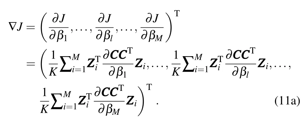
The basic idea of the ETS in this paper is to use the sensitivity(gradient)of forecasterror variance over the verification region in terms of analysis error variance to determ ine data sensitive regions foradaptiveobservations.It is the fi rst order approximation of Eq.(10),but only a single transformation matrix computation w ill be needed,thus improving computation efficiency when compared to ET.Themain objective is to derive amathematical formulation of∂J/∂βlin this paper.

Follow ing Eq.(8),the gradientof J to the analysis error variance reduction ratioβis

Theestimated forecasterror variance reduction is

In the BT1999 implementation,dβis set to a constant w ith a value of 0.5.The ETmethod isapproximated by ETS derivatives.In operationalapplications,Δβcan be set to differentvaluesatdifferent locations thatcan really takeadvantage of an analysis error covariance,e.g.,a large reduction (Δβ)occursovera largeanalysiserror variance.

3.2. Derivatives of the transformationmatrix C formulation

Themain contribution of the ETSmethod is the derivation of an analytic gradient formulation of∂CCCCCCT/∂βin Eq. (11a)in termsof theerror reduction coefficientβl.

For the ET transformation matrix CCC,let us introduce a matrix

and then the product of ET transformation matrix CCCCCCT= KΨ−1as given in Eq.(6).Using an inversematrix derivative formulation,the ET transformation productderivative is,

where,

Thus,ET sensitivity can beobtained using Eqs.(11–14).

Note the∂AAAg/∂βlis usually a constantmatrix.For an example of a diagonalmatrix of AAAg=diag(α1β1,...,αMβM) (BT1999),∂AAAg/∂βl|β=1is equal to a diagonal matrix of diag(0,...,0,αl,0,...,0).For a given guessed analysis error variance AAAg,the ET transformationmatrix CCCCCCTis determ ined.So the ET sensitivity from Eq.(15)can be obtained aftera single computation of a transformationmatrix instead of calculating ensemble transformations(CCC[β]CCCT[β])for all possible perturbations in ET using Eq.(10).

3.3. Practicalprocedure and computation cost

When applying ETS in practice,Eq.(15)is not solved directly.Hereare the implementation procedures:

Step 1:Compute theperturbation fieldsatthe tfa:XXXe(tfa), and tv:XXXe(tv).

Step 2:Initial the projection matrix℘and the guessed analysiserrorvariance AAAg.

Step 3:Compute the inverse of Eq.(12): XXX e(tfa)T AAA−1g XXX e(tfa)

Step 4:Compute thematrix ZZZ:ZZZ=XXXe(tv)T℘

Step 5:Obtain all the signals[Eq.(11a)]:∂J/∂βl,l= 1...M.Decompositionof the K×K symmetricmatrix(CCCCCCT) takes K3/6 computing operations(Step 3 costs～K3/6).In order to obtain allof thesensitivity,ETSneeds to estimate the sensitivity atall the elements in the state vector(M),w ith an Eq.(11a)costof～M2(Step 5 costs～M2).So,thecomputation countof ETS isabout M2+K3/6.However,ET needs to decompose the CCCCCCTmatrix ateach elementin thestatevector [Eqs.(9)and(10)w ith a costof～M2+K3/6]to obtain allthe signals(forecasterror reduction).Themagnitude of K is about102.The Mis103in a very coarse resolution.Itcould rise to 108in thehigh-resolution case.Table2 shows theestimation of the computation countsof ET and ETS.ETSgains greatly in efficiency as itonly needs to decompose the CCCCCCTonce.When Mand K are large,thedifference issignificant.

Table 2.Estimated computation countsof ET and ETS.

4. Numericalexperiments

In thissection,weapply ETand ETS forahurricane case and a rainfall case.The fi rst case,Hurricane Irene(2011), formed on 21 August,and became a hurricane on 22 August 2011.It then passed Exuma and Cat Islands.Itmade landfall near Cape Lookout,North Carolina at1200UTC on 27 August.It continued tracking north northeastward,andmoved over Manhattan,New York on 28 August.The heavy rainfalland strong w ind caused severe damage(Avila and Stewart,2012).We also apply ET and ETS for a heavy rainfall case.The heavy precipitation in this case is associated with a low level vortex that developed overwestern China during 3-5 August 2013.The hourly accumulate precipitation was＞30mm over the Beijing areasat1200UTC 4August2013.

4.1. Data and experimentsetup

The European Centre for Medium-range Weather Forecastsensemble forecastsare used in thisstudy,which can be downloaded from the THORPEX Interactive Grand Global Ensemble(TIGGE)portal(http://apps.ecmw f.int/datasets/ data/tigge/).The initial time of the ensemble forecasts are at0000UTC 24August2011 and 1200UTC 3 August2013 for the hurricane and heavy rainfall case,respectively.The length of prediction time is 72-h w ith a 6-h interval for the ensemble prediction outputs.The variables selected for the ET dry energy norm are the temperatureand horizontalw ind componentsat the850,500 and 200 hPapressure levels.The diagonalvaluesof guessed analysiserror covariance AAAgused are the same as ETKF(Majumdar etal.,2002):the guessed analysiserror covarianceofw ind at the850,500 and 200 hPa pressure levels is 2.72,3.16 and 4.66m s−1separately;the guessed analysis error vovariance of temperature at the 850, 500 and 200 hPa pressure levels is 1.22,0.92°C and 1.82°C separately.

For the hurricane case,the verification area(26°–40°N, 86°–70°W)ismarked by the inner rectangle showed in Fig. 1a).The estimation or potential targeting observation area is the whole domain(10°–50°N,100°–60°W).The ensemblemean indicated that the hurricane wasmoving towards the east coastof the U.S.at 0000 UTC 27 August,and it is selected as the tvin this case.Thereareseven tfafor theadaptive observations,−0 h,−12 h,−24 h,−36 h,−48 h,−60 h,and−72 h.The negative hours tfaindicate the number of hoursahead of the tv,correspondingly.For the heavy rainfall case,the verification area isover the Beijing area(38°–42°N, 114°–120°E),(Fig.1b).The estimation potential targeting area was covered from 100°E to 124°E and 34°N to 50°N. The tvis the heavy rainfall time,1200 UTC 4 August2013. The tfaare set to 6 h and 12 h ahead of the tv.As claimed in section3,ETSismoreefficientwhen thenumberofensemble members(K)and the elements in state vectors(MMM)aremathematically large.We set up six experiments(Table 3)w ithdifferent resolutions and ensemblemembers to demonstrate this claim numerically.The number of ensemblemembers vary from 10 to 30 to 50.Two resolutions are used,1°×1°and 2°×2°.As an example,K30R1 means the number of ensemblemembers is30 and the resolution is1°×1°.

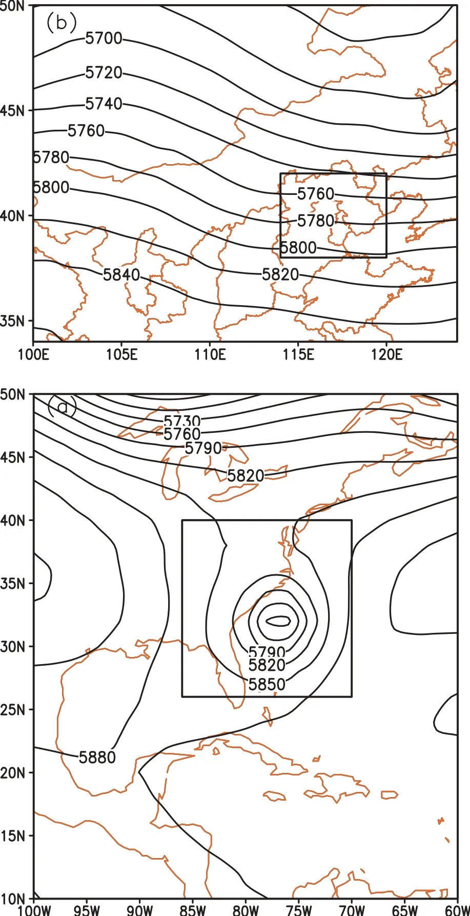
Fig.1.The domain and verification areas for the(a)Hurricane Irene(2011)and(b)Beijing rainfallcases.Contoursare theensemblemean geopotentialheightat500 hPa(gpm).The inner rectangle is the verification areas.

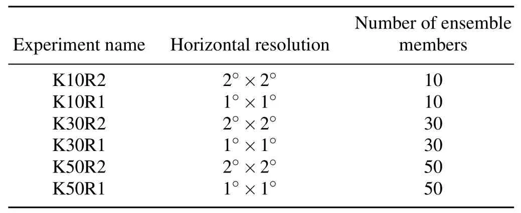
Table 3.Setup of numerical Experiments.

4.2. Summarymap

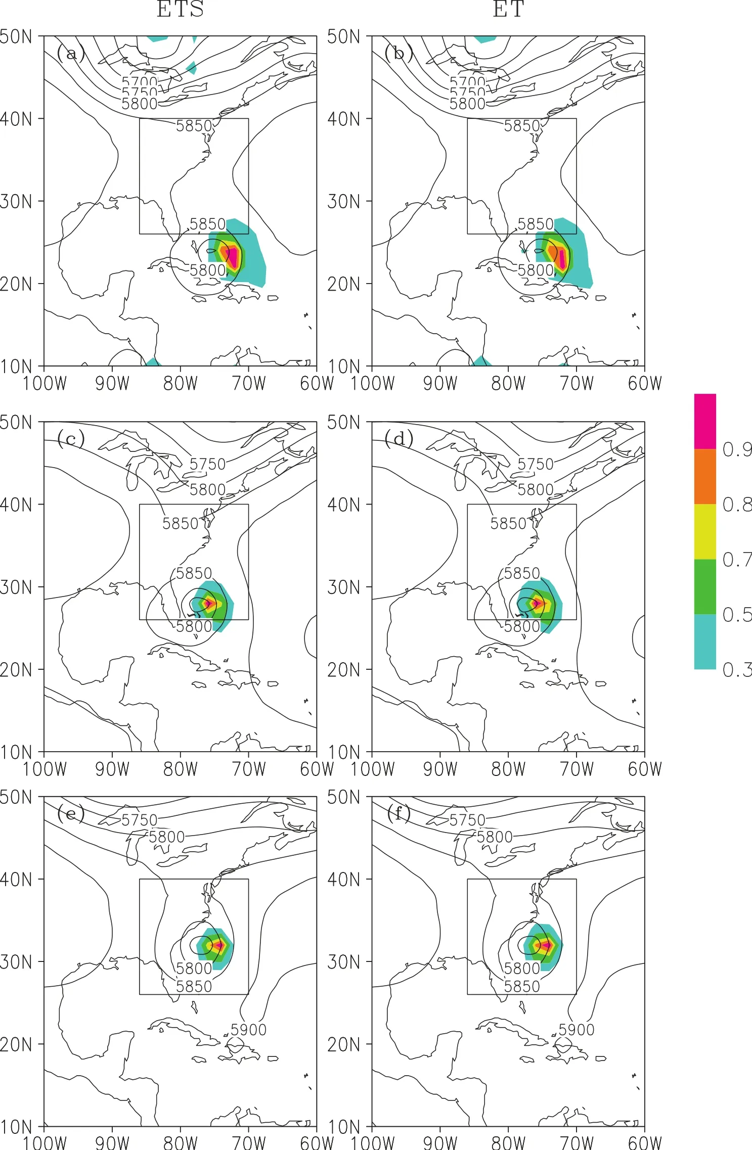
Fig.2.The signals(color fi lled areas)identified by(a,c,e)ETS and(b,d,f)ET at a different tain K30R2 for the Hurricane Irene case.The taare(a,b)0000 UTC 25 August;(c,d)0000 UTC 26 August,(e,f)0000 UTC 27 August.The contours are the 500 hPa geopotential heightof the ensemble mean forecastateach ta.The inner rectangle is the verification area.The tvis0000UTC 27 August.

A summarymap—the signalsof sensitivity identified by ET or ETS over the whole calculation domain—shows the sensitive area.ET considered each grid pointas a hypothetical adaptive site and identified sensitive areas by perturb-ing the analysis error variance ateach observation site.The signal—the reduction of forecasterror covarianceassociated w ith this grid point—can be obtained.The summary map can be plotted after perturbing the variance and calculating the reduction overall thegrid points.

In contrast to these perturbationsof ET,the ETSmethod can obtain thesevaluesby asingle computation of thederivative,using the same amount of computation as would be needed for each individual ET perturbation.The derivatives areshown,aswellas the reduction ofanalysiserrorvariance. They represent the sensitivity signalsover the calculation domain.

In order to compare the signals from ETSand ET atdifferent tfa,the signals from Eqs.(10)and(15,11b)are normalized in thisstudy, where Smax/Sminare themaximum/minimum valuesover the whole domain.Thus,the summary maps show the relative sensitivity of the ET or ETSmethods.

4.3. Sensitive areas identified by ET and ETS

The color fi lled areasof Fig.2 show the normalized signals identified by ET and ETS at different tfafor experiment K30R2 in the hurricane case.Itisseen thatETSand ET give similar signal patternsand evaluation.As the tfaapproached the tv,the signal(color fi lled contour areas)approached the verification areas.Thesensitivity areasaredistributed around the hurricane itself,and evolved into the verification areasat the tv.Figure3 shows thenormalized signals identified from ET and ETS from K50R2 and K10R1.The results are very close to K30R2.The signals are both located at the hurricane’s eastern center.It shows that the data sensitive region identified by ETS is very close to ET even when the resultsare from a different number of ensemblemembers and resolutions.Generally,the ETS can obtain the same sensitive areasas ETw ithouthigh consumption.

Fig.3.The signals(color-fi lled areas)identified by(a,c)ETS and(b,d)ET in the Hurricane Irene case:(a,b)are Experiment K50R1;(c,d)experiment K10R2.The tais 0000 UTC 26 August2011.The contoursare the 500 hPa geopotentialheightofensemblemean forecasts.

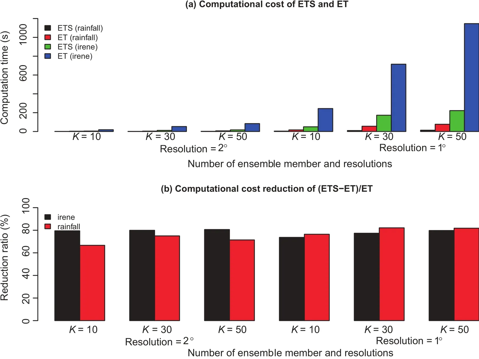
Fig.4.(a)Computational costof differentexperiments.(b)Relative computation time reduction.

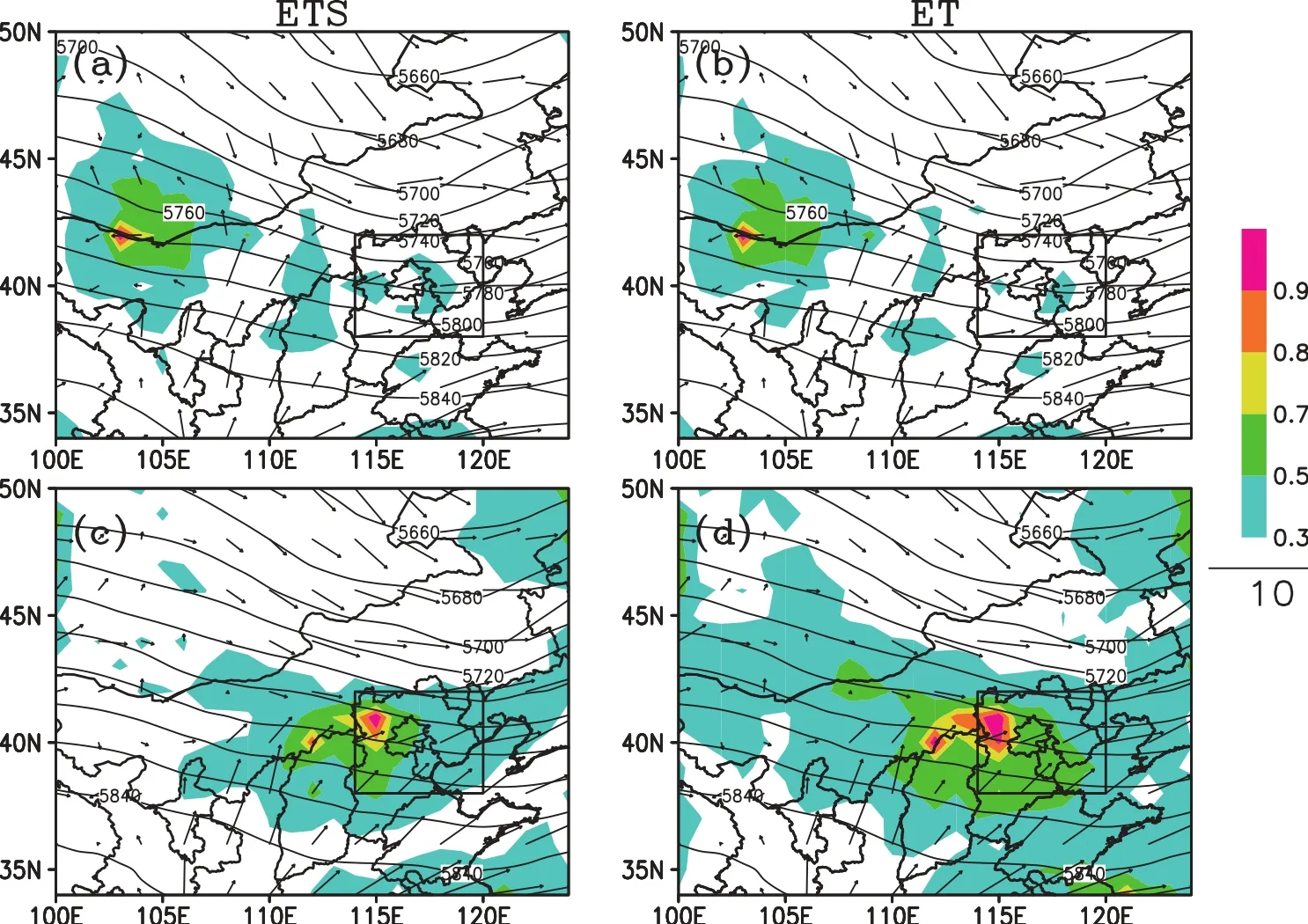
Fig.5.The signals(color fi lled areas)identified by(a,c)ETSand(b,d)ET in K30R2 for the Beijing rainfall case.The tvis 1200 UTC 4 August 2013.The taare(a,b)is 0000 UTC 4 August;(c,d) 0600 UTC 4 August.The w ind barbs are the horizontalw ind componentat850 hPa(units:m s−1). The contours are the 500 hPa geopotentialheightof the ensemblemean forecastateach t a.The inner rectangle is the verification area.

ETS ismuch faster than ET because ET needs to loop over all the possible elements in the state vector(M),especiallywhen thenumberofensemblepredictionmembers(K) is large.Figure 4 shows the computational costs and relative computation time reduction w ith ETS and ET using a differentnumber of ensemble predictionmembers(K).The cost is less than 60 secondsw ith a fine resolution and few ensemble prediction members for ETS and ET.This is acceptable for the adaptive observations.However,the computational cost rises to about 1200 seconds w ith a 1°×1°resolution in the horizontaldirection,w ith three vertical levels and 50 ensemble prediction members.ETS only costs about 200 seconds.Overall,the computation time saved by ETwas60%–80%(Fig.4b).If the computational domain is larger(particularly foraglobalmodel)w ith higher resolution in the horizontal and vertical directions(here the computationswere conducted in three vertical levelsonly),the reduction in computational costswould bemuchmore significant w ith ETS compared to ET.

Thesignals from theheavy rainfallcaseare shown in Fig. 5.Itcan be seen that the signalsare similarbetween ET and ETS.The sensitive areas were distributed around the w ind divergence(850 hPa)and the trough(500 hPa)at 12 hours ahead of the tv(Figs.5aand b).The signalsare located in the westof the verification areasat6 hoursahead of the tv(Figs. 5c and d).Although the sensitive areas from the ET covered a slightly larger area compared to ETS,signals w ith maximum values are located at almost the same position in ET and ETS.The follow ing section providesmore discussion on thedifferencesbetween ETSand ET.

4.4. Differencesbetween ET and ETS

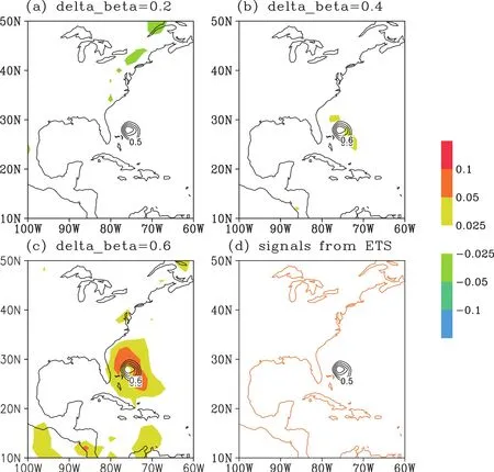
Fig.6.The signals for the Hurricane Irene(2011)case.Contoursare the signals from(a–c)ET and(d) ETS.TheexperimentisK30R2.The tais0000UTC 26August2011.Color fi lled areasshow thesignal differencesbetween ETSand ET.Theanalysiserror reduction for ET is(a)0.2,(b),0.4 and(c)0.6.

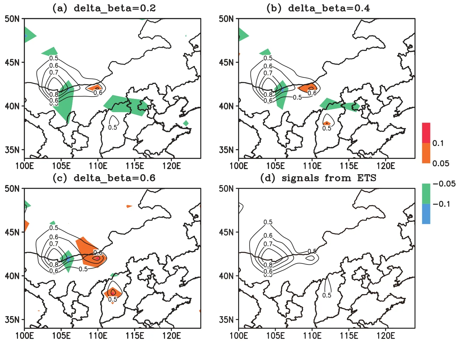
Fig.7.As in Fig.6 but for the rainfall case.The tais0000UTC 4August2013.

In BT1999,the signals are calculated by Eq.(10).ETS used Eq.(15)to calculate the signals.So ETS is a fi rst order approximation of the ET.This also means the results from ETS should get closer to those of ET whenΔβapproaches zero.Herewe setup threemore numericalexperimentsusing differentΔβvalues for ET(Δβ=0.2,0.4,0.6). WhenΔβ=0.2 thismeans the ET signals are estimated by: sl=J[βl=1]−J[βl=0.8]It isnoted thatETSsignals[Eqs. (10a),(14)]do not vary w ith differentΔβ.Figures 6 and 7 show the ETSand ET signals for the Hurricane Irene(2011) and Beijing rainfall cases,respectively.The differences between ETSand ET are presented by the color shading colors. It is seen that for the smallestΔβ,the twomethods produce almost the same data sensitive region(Figs.6 and 7).And for larger values ofΔβ,the ETS signal distribution is still close to the ET signal;in particular,the centersof the signals from the twomethodsare almost the same evenw ith a large Δβ.Overall,for the Hurricane Irene(2011)case,both ET and ETS identify one sensitive region(Fig.6);for the rainfall case,one region w ith globalmaximum signals and two local regionsw ith localmaximum signals(Fig.7)are identified.The differencesbetween ET and ETS are acceptable, since the targeting observation focuseson the sensitive areas w ith amaximum(the center of the signals).Generally the signals from ET and ETSaresimilar.

5. Conclusion and discussion

Adaptive observations have the potential to improve weather forecasts.Among existing methods of identifying observation sensitivity regions,ET isattractivebecauseof its useofanalysiserror covariance information and itsefficiency compared to othermore complex methods.In this study,a new ly proposed ETS approach for adaptive observations is derived and demonstrated.The ETSmethod only usesa singlecomputation ofa transformationmatrix to yield asensitivity summary map,instead of calculating ensemble transformations for all possible perturbations,as in the ETmethod. Thus,it further increase the computationalefficiency.If the computationaldomain is larger(even global in thehorizontal direction),w ith higher resolution in the horizontal and vertical directions,the reduction in computational cost would be far greaterw ith ETS compared to ET.Numericalexperimentsw ith Hurricane Irene(2011)and a heavy rainfall case in Beijing showed thatETS reduced the computation costby 60%–80%.

Thesummarymaps from the two casesshow thattheETS method produces a similar data sensitive region as the ET method,especially for the region w ith large signal values. Thus,the new method gains computational efficiency w ithout losing the positive characteristicsof the ETmethod.It is noted that,in general,themore realistic the analysis covariance is,thebetter the targeting region is thatcan be identified under the assumption of ET.As themain aim of this paper is mainly to introduce the ETSmethod,thebestguessofanalysis covariance,which can be provided by a data assimilation system(e.g.,ETKF),w ill be further studied in future work. Our plan is to implement ETS at the NCEP Environmental Modeling Center for WSR,and compare it to the existing ET adaptive observation method in future works.With its improved efficiency,ETS can be applied to severe weather eventsw ith high spatial resolution and a large number of ensemblemembers.

Acknow ledgements.The authors thank John C.OSBORN at NOAA Earth System Research Laboratory for his English editorial supporton thismanuscript.The authorswould like to express their appreciation to the two anonymous reviewers for their commentson theearlierversion of themanuscript,which helped improve thepresentation of this paper.Thiswork was jointly sponsored by the Key Projectof theChineseNationalPrograms for FundamentalResearch and Development(“973Program”,GrantNo.2013CB430106),andthe Key Projectof the Chinese National Science&Technology Pillar Program during the Twelfth Five-year Plan Period(Grant No. 2012BAC22B01).

REFERENCES

Aberson,S.D.,2003:Targeted observations to improve operational tropical cyclone track forecast guidance.Mon.Wea. Rev.,131,1613–1628.

Aberson,S.D.,S.J.Majumdar,C.A.Reynolds,and B.J.Etherton,2011:An observing system experiment for tropical cyclone targeting techniques using the global forecast system. Mon.Wea.Rev.,139,895–907.

Ancell,B.,and G.J.Hakim,2007:Comparing adjoint-and ensemble-sensitivity analysisw ith applications to observation targeting.Mon.Wea.Rev.,135,4117–4134.

Anderson,J.L.,1997:The impactof dynamical constraintson the selection of initial conditions for ensemble predictions:Low orderperfectmodel results.Mon.Wea.Rev.,125,2969–2983.

Avila,L.A.,and S.Stewart,2012:Atlantic hurricanes 2011:A ll about Irene and Lee.Weatherwise,65,34–41.

Bauer,P.,R.Buizza,C.Cardinali,and J.-N.Th´epaut,2011:Impactof singular vector based satellite data thinning on NWP. Quart.J.Roy.Meteor.Soc.,137,286–302.

Berger,H.,R.Langland,C.S.Velden,C.A.Reynolds,and P. M.Pauley,2011:Impact of enhanced satellite-derived atmosphericmotion vector observations on numerical tropical cyclone track forecasts in the western North Pacific during TPARC/TCS-08.J.Appl.Meteor.Climatol.,50,2309–2318.

Bishop,C.H.,and Z.Toth,1999:Ensemble transformation and adaptive observations.J.Atmos.Sci.,56,1748–1765.

Bishop,C.H.,B.J.Etherton,and S.J.Majumdar,2001:Adaptive sampling w ith the ensemble transform Kalman fi lter.Part I: Theoreticalaspects.Mon.Wea.Rev.,129,420–436.

Buizza,R.,and A.Montani,1999:Targeted observations using singular vectors.J.Atmos.Sci.,56,2965–2985.

Chang,E.K.M.,M.H.Zheng,and K.Raeder,2013:Mediumrangeensemble sensitivity analysisof two extreme pacific extratropical cyclones.Mon.Wea.Rev.,141,211–231.

Chou,K.-H.,C.-C.Wu,P.-H.Lin,S.D.Aberson,M.Weissmann, F.Harnisch,and T.Nakazawa,2011:The impact of dropw indsonde observations on typhoon track forecasts in DOTSTAR and T-PARC.Mon.Wea.Rev.,139,1728–1743.

Ehrendorfer,M.,R.M.Errico,and K.D.Raeder,1999:Singularvectorperturbation grow th in aprimitiveequationmodelw ith moistphysics.J.Atmos.Sci.,56,1627–1648.

Ham ill,T.M.,J.S.Whitaker,and C.Snyder,2001:Distancedependent fi ltering of background error covariance estimates in an ensemble Kalman fi lter.Mon.Wea.Rev.,129,2776–2790.

Ito,K.,and C.-C.Wu,2013:Typhoon-position-oriented sensitivity analysis.Part I:Theory and verification.J.Atmos.Sci.,70, 2525–2546.

Joly,A.,and Coauthors,1997:The frontsand Atlantic storm-track experiment(FASTEX):Scientific objectives and experimentaldesign.Bull.Amer.Meteor.Soc.,78,1917–1940.

Joly,A.,and Coauthors,1999:Overview of the field phase of the fronts and Atlantic Storm-Track EXperiment(FASTEX) project.Quart.J.Roy.Meteor.Soc.,125,3131–3163.

Langland,R.H.,R.Gelaro,G.D.Rohaly,and M.A.Shapiro, 1999a:Targeted observations in FASTEX:Adjoint-based targeting proceduresand data impactexperiments in IOP17 and IOP18.Quart.J.Roy.Meteor.Soc.,125,3241–3270.

Langland,R.H.,and Coauthors,1999b:The North Pacific experiment(NORPEX-98):Targeted observations for improved North American weather forecasts.Bull.Amer.Meteor.Soc., 80,1363–1384.

Majumdar,S.J.,C.H.Bishop,B.J.Etherton,I.Szunyogh,and Z. Toth,2001:Can an ensemble transform Kalman fi lter predict the reduction in forecast-error variance produced by targeted observations?Quart.J.Roy.Meteor.Soc.,127,2803–2820.

Majumdar,S.J.,C.H.Bishop,B.J.Etherton,and Z.Toth,2002: Adaptive sampling w ith the ensemble transform Kalman fi lter.Part II:Field program implementation.Mon.Wea.Rev., 130,1356–1369.

Majumdar,S.J.,and Coauthors,2011:Targeted observations for improving numerical weather prediction:An overview. WWRP/THORPEX No.15.

Mu,M.,F.F.Zhou,and H.L.Wang,2009:A method for identifying the sensitive areas in targeted observations for tropical cyclone prediction:Conditional nonlinear optimal perturbation.Mon.Wea.Rev.,137,1623–1639.

Palmer,T.N.,R.Gelaro,J.Barkmeijer,and R.Buizza,1998:Singular vectors,metrics,and adaptive observations.J.Atmos. Sci.,55,633–653.

Szunyogh,I.,Z.Toth,R.E.Morss,S.J.Majumdar,and C.H. Bishop,2000:The effectof targeted dropsonde observations during the 1999 w inter storm reconnaissance program.Mon. Wea.Rev.,128,3520–3537.

Szunyogh,I.,Z.Toth,A.V.Zim in,S.J.Majumdar,and A.Persson,2002:Propagation of theeffectof targeted observations: The 2000 w inter storm reconnaissance program.Mon.Wea. Rev.,130,1144–1165.

Wang,H.L.,M.Mu,X.Y.Huang,2011:Application of conditional non-linear optimal perturbations to tropical cyclone adaptive observation using the weather research forecasting (WRF)model.Tellus A,63,939–957.

Wu,C.-C.,K.-H.Chou,P.-H.Lin,S.D.Aberson,M.S.Peng,and T.Nakazawa,2007a:The impactof dropw indsonde data on typhoon track forecasts in DOTSTAR.Wea.Forecasting,22, 1157–1176.

Wu,C.-C.,J.-H.Chen,P.-H.Lin,and K.-H.Chou,2007b:Targeted observationsof tropicalcyclonemovementbased on the adjoint-derived sensitivity steering vector.J.Atmos.Sci.,64, 2611–2626.

Wu,C.-C.,S.-G.Chen,J.-H.Chen,K.-H.Chou,and P.-H.Lin, 2009:Interaction of Typhoon Shanshan(2006)w ith them idlatitude trough from both adjoint-derived sensitivity steering vector and potential vorticity perspectives.Mon.Wea.Rev., 137,852–862.

Xie,B.G.,F.Q.Zhang,Q.H.Zhang,J.Poterjoy,and Y.H.Weng, 2013:Observing strategy and observation targeting for tropical cyclones using ensemble-based sensitivity analysis and dataassimilation.Mon.Wea.Rev.,141,1437–1453.

23 January 2015;revised 11May 2015;accepted 15 June 2015)

:Zhang,Y.,Y.F.Xie,H.L.Wang,D.H.Chen,and Z.Toth,2016:Ensemble transform sensitivity method for adaptive observations.Adv.Atmos.Sci.,33(1),10–20,

10.1007/s00376-015-5031-9.

∗Corresponding author:Yuanfu XIE

E-mail:yuanfu.xie@noaa.gov