A Timescale Decomposed Threshold Regression Downscaling Approach to Forecasting South China Early Summer Rainfall

Linye SONG,Wansuo DUAN,Yun LI,and Jiangyu MAO00089

2State Key Laboratory of Numerical Modeling for Atmospheric Sciences and Geophysical Fluid Dynamics, Institute of Atmospheric Physics,Chinese Academy of Sciences,Beijing100029

3Business Intelligence&Data Analytics,Western Power,Perth WA6000,Australia

A Timescale Decomposed Threshold Regression Downscaling Approach to Forecasting South China Early Summer Rainfall

Linye SONG1，2,Wansuo DUAN∗2,Yun LI3,and Jiangyu MAO2
1Institute of Urban Meteorology,China Meteorological Administration,Beijing100089

2State Key Laboratory of Numerical Modeling for Atmospheric Sciences and Geophysical Fluid Dynamics, Institute of Atmospheric Physics,Chinese Academy of Sciences,Beijing100029

3Business Intelligence&Data Analytics,Western Power,Perth WA6000,Australia

(Received 3 December 2015;revised 4 April 2016;accepted 4 May 2016)

A timescale decomposed threshold regression(TSDTR)downscaling approach to forecasting South China early summer rainfall(SCESR)is described by using long-term observed station rainfall data and NOAA ERSST data.It makes use of two distinct regression downscaling models corresponding to the interannual and interdecadal rainfall variability of SCESR. The two models are developed based on the partial least squares(PLS)regression technique,linking SCESR to SST modes in preceding months on both interannual and interdecadal timescales.Specifically,using the datasets in the calibration period 1915–84,the variability of SCESR and SST are decomposed into interannual and interdecadal components.On the interannual timescale,a threshold PLS regression model is fitted to interannual components of SCESR and March SST patterns by taking account of the modulation of negative and positive phases of the Pacific Decadal Oscillation(PDO).On the interdecadal timescale,astandard PLSregression model is fittedtothe relationship between SCESRand preceding November SST patterns.The total rainfall prediction is obtained by the sum of the outputs from both the interannual and interdecadal models.Results show that the TSDTR downscaling approach achieves reasonable skill in predicting the observed rainfall in the validation period 1985–2006,compared to other simpler approaches.This study suggests that the TSDTR approach, considering diff erent interannual SCESR-SST relationships under the modulation of PDO phases,as well as the interdecadal variability of SCESR associated with SST patterns,may provide a new perspective to improve climate predictions.

timescale decomposed threshold regression,South China early summer rainfall,forecasting skill

1. Introduction

An important task for fl ood and drought management is the provision of accurate rainfall prediction.The rainfall distribution in China is generally characterized by a“southern fl ood and northern drought”pattern,due to the weakening of the East Asian summer monsoon after the late 1970s(Nitta and Hu,1996;Wang,2001;Gong and Ho,2002).Accompanied by the northward seasonal march of the East Asia summer monsoon,abundant rainfall first appears over South China(SC)in mid-May(Tao,1987;Lau and Weng,2001; Ding et al.,2008;Wu et al.,2012),and leads to the peak of annual rainfall in early summer(June)over the region (Fig.1a).Because SC is one of China’s largest economic zones with a large population,extreme fl ood events in early summer often cause a large number of human casualties and considerable economic loss(Chan and Zhou,2005;Zhou et al.,2006).Thus,improving seasonal forecasting skill for early summer rainfall over SC is of great importance for disaster prevention and mitigation.

There are several approaches to forecasting rainfall.One is using numerical models(e.g.Collischonn et al.,2005; Aligo et al.,2009).The raw model prediction is dynamically meaningful,but still has low skill for many reasons;for instance,because of the model resolution(Martin,1999),subgrid processes(Grotch and MacCracken,1991)and parameterization schemes(Eitzen and Randall,1999).Hence,precipitation modeling is regarded as one of the most difficult issues in climate modeling,resulting in low skill on the basis of the pure numerical approach.Another approach to forecasting rainfall is based on statistical downscaling models (Liu and Fan,2012a,2014;Sun and Chen,2012).A statistical downscaling method combining the GCM-simulated and observed information is developed,which shows much better predictabilityforglobalprecipitationforecasting(SunandChen,2012).In addition,pure statistical downscaling models are also used to forecast rainfall.The method is generally based on an empirical observed relationship between the large-scale climate anomalies and local rainfall fl uctuations. Therearevariousmethodsthatcanbeusedtodevelopstatistical downscaling models,including multiple linear regression (Wilby,1998),principle components(Liand Smith,2009), and singular value decomposition(Zhu et al.,2008;Liu and Fan,2012b).Other more sophisticated methods include partial least squares(PLS)regression(Zhang et al.,2011;Wu et al.,2013).

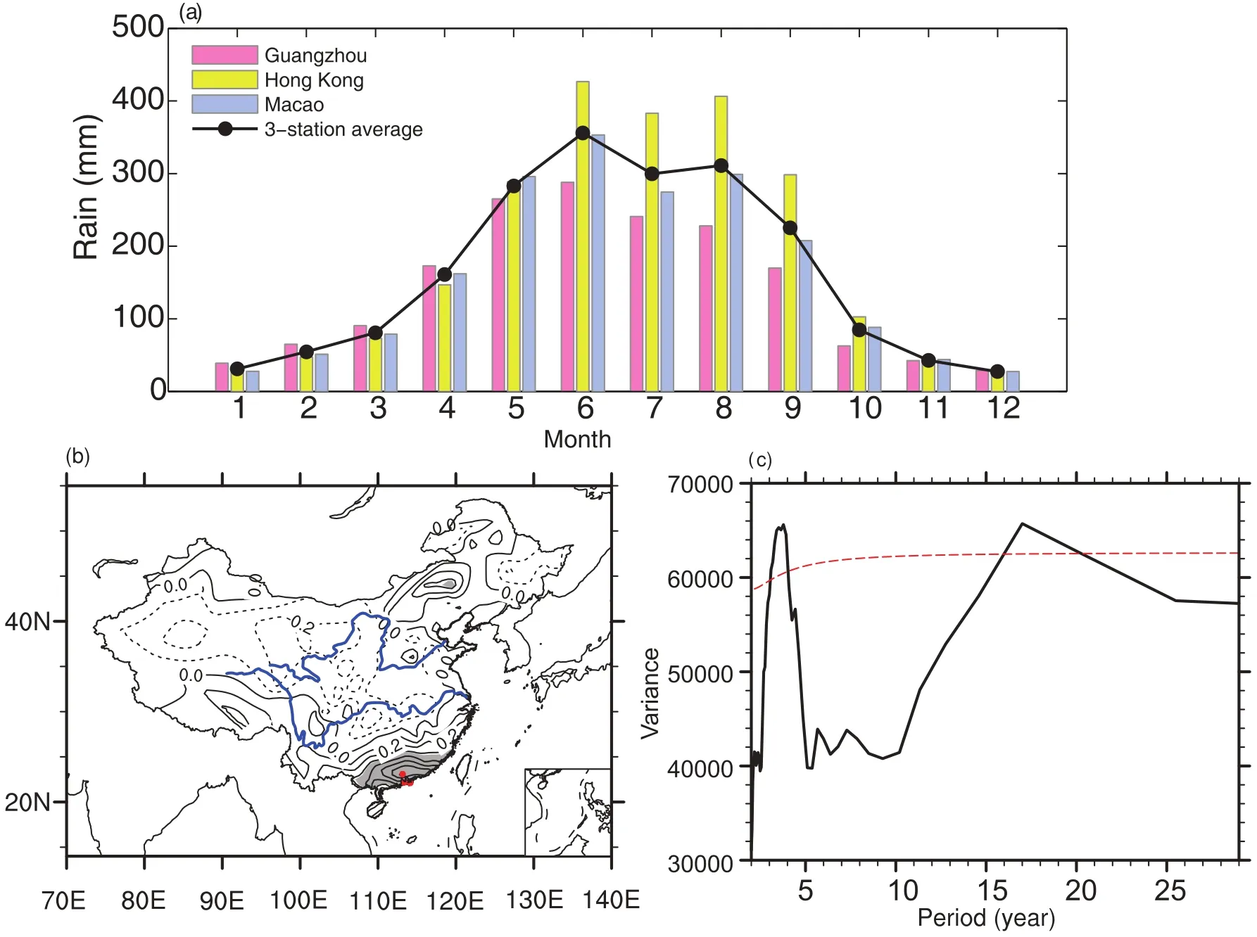
Fig.1.(a)The annual climatological cycle of the rainfall at the stations of Guangzhou,Hong Kong and Macao,as well as the 3-station average,during 1910–2011.(b)Detrended correlation of the 3-station averaged rainfall with the 160-station rainfall from CMA in June during 1951–2011.The stations at Guangzhou,Hong Kong and Macao are indicated by the three red dots.The grey shading indicates CCs significant at the 99%con fidence level based on the t-test,presenting the SC region.(c)Power spectrum for June rainfall.The peak over the red dashed line indicates the con fidence level is greater than 80%against red noise.

Pure statistical downscalingmodels show reasonable skill in predicting regional rainfall.For example,Sahaiet al. (2003)made optimum use of global SST for Indian summer monsoon rainfall prediction nine months in advance. Rainfall may contain variabilities on various timescales,with low-frequency interdecadal variability associated with pronounced wetting or drying trends(Ding et al.,2008)and high-frequencyinterannualvariabilityrelatedtosevere fl oods or droughts(Huang et al.,2006).Guo et al.(2012)described a timescale decomposition(TSD)approach to statistically downscale the late summer rainfall over North China,which made use of two distinct downscaling models corresponding to the interannualandinterdecadalrainfall variability,respectively.However,the TSD approach by Guo et al.(2012)neglected the possibility that the interannual rainfall variability may be modulated by an interdecadal climatic background.

Recently,an increasing number of studies have suggested that the interannual relationships of large-scale climate anomalies with local or remote climate fl uctuations are not stationary(e.g.Torrence and Webster,1999;Wang,2002; Wu and Wang,2002;Gao et al.,2006;Sun and Wang,2012; Chen et al.,2013a;Chen et al.,2015a,2015b;Cao et al., 2015,2016).In particular,the modulation of a decadal-scale coupled ocean atmospheric mode named the Pacific Decadal Oscillation(PDO)(Mantua et al.,1997;Mantua and Hare, 2002)has attracted more attention in the last decade(Gershunov and Barnett,1998;Power et al.,1999;Chan and Zhou,2005;Wang et al.,2008;Mao et al.,2011;Chen et al., 2013b;Duanetal.,2013).Forexample,it has beenfoundthat the typical in fl uences of ENSO on the North American climate are strong and consistent only during preferred phasesof the PDO(Gershunov and Barnett,1998).The ENSO–East Asian summer monsoon relationship during 1962–77 has been found to be significantly diff erent from that during 1978–93(Wu and Wang,2002),which is actually consistent with a phase transition from negative to positive PDO in the late-1970s.In the SC region,the interannual rainfall variation has also been suggested to be modulated by the PDO(Chan and Zhou,2005;Mao et al.,2011;Duan et al., 2013).Ithasbeenproposedthatincorporatinginformationon the PDO could improve the long-term predictability of early summer SC rainfall changes(Chan and Zhou,2005;Zhou et al.,2006).Therefore,a statistical model that takes into account the modulation of the PDO may lead to better skill in seasonal rainfallpredictionoverSC.This naturallyraises two key questions:How can the modulatione ff ect of the decadalscale coupled oceanic–atmospheric mode of the PDO be incorporated when developing a statistical downscaling model to forecast the early summer rainfall over SC?And can the forecasting skill be improved?

The aim of this paper is to describe a TSD threshold regression(TSDTR)downscaling approach for the statistical forecasting of South China early summer rainfall(SCESR). The TSDTR downscaling approach includes two distinct regression downscaling models,called the interannual model (IAM)and interdecadal model(IDM),respectively linking SST patterns prior to early summer to the interannual and interdecadal variability of SCESR.On the interannual timescale,the IAM,based on a threshold PLS regression model,is fitted to interannual components of SCESR and March SST patterns by taking account of the modulation of negative and positive phases of the PDO.On the interdecadal timescale,the IDM,based on a PLS regression model,is employed to fit the relationship between SCESR and preceding November SST patterns.The total rainfall prediction is obtained bythesum ofthe outputsfromboththe IAMandIDM.

The rest of this paper is arranged as follows:Section 2 introduces the datasets used in this work.The TSDTR downscaling approach is described in section 3.Results of the TSDTR approachin forecastingSCESR are presentedin section 4.Section 5 is a summary and discussion.

2. Data

Long-term reliable observed rainfall data are derived from the monthly rain gauge datasets from three stations:Hong Kong(22.11°N,114.14°E),Macao(22.16°N, 113.35°E)and Guangzhou(23.08°N,113.16°E).These rainfall data have been used by previous studies(Chan and Zhou, 2005;Mao et al.,2011;Duan et al.,2013)and are chosen here because of their long-term reliability since 1910.The maximum rainfall of these three stations occurs in June(Fig. 1a),which purely belongs to the South China Sea summer monsoon rainfall(Tao,1987;Wang et al.,2004).Another set of monthly rainfall data derived from 160 Chinese meteorological stations provided by the China Meteorological Administration(CMA)is also used in this study,available from 1951.The simultaneous correlation pattern of three-station averaged rainfall in June with the 160-station rainfall from CMA duringtheperiod1951–2011showssignificantpositive correlationover the region of SC(Fig.1b).Thus,it is reasonable to use the long-term,high-quality three-station(Hong Kong,Macao and Guangzhou)averaged rainfall in June to represent the SCESR in this study.

The PDO index,de fined as the leading EOF of SST anomalies in the North Pacific Ocean poleward of 20°N after removing the global warming signal(Mantua et al.,1997; Mantua and Hare,2002),is taken from the website of the Joint Institute for the Study of the Atmosphere and Ocean (http://jisao.washington.edu/pdo/PDO.latest),which contains data from 1900 onward.An 11-year running mean of wintertime(October–March averaged)PDO index is used to obtain the interdecadal variability of the PDO(Mantua and Hare, 2002;Mao et al.,2011)over the period 1910–2011(Fig.2a). Note that10 yearsare missing,caused bythe 11-yearrunning mean,and thus the period for the forecasting experiment in this work is chosen as 1915–2006.Monthly SST data are extracted from NOAA ERSST.v3b(Smith and Reynolds,2004; Smithet al.,2008)on2.0°×2.0°grid,which is availablefrom the year 1854 at http://www.esrl.noaa.gov/psd/data/gridded/. Monthly atmospheric data are obtained for the period from 1948 from the NCEP–NCAR reanalysis products on 2.5°× 2.5°grid(Kalnay et al.,1996),including horizontal winds and specific humidity at diff erent levels(also available at http://www.esrl.noaa.gov/psd/data/gridded/).

3. Methods

Two primary peaks with periods of about 4 years and 17 years exist in the SCESR,as determined by spectrum analysis(Fig.1c),indicatingapparent interannualand interdecadal variability.Therefore,the observed time series of total rainfall(RainT)is decomposed into interannual(variation less than 11 years,denoted as RainA)and interdecadal(variation longer than 11 years,denoted as RainD)components by an 11-year high-pass and low-pass filter(Fig.2b).That is, RainT=RainA+RainD.

SST anomalies have been found to be important in in fl uencing the East Asian climate(Huang and Wu,1989;Wang et al.,2000;Lau and Weng,2001;Wu et al.,2012),have a relatively long“memory”(Sahaiet al.,2003),and can therefore be regarded as a preceding predictor for SCESR.This motivates us to explore the relationships between SCESR and associated SST patterns on both interannual and interdecadal timescales.As such,we also decompose the SST field into interannual(SSTA)and interdecadal(SSTD)components.To revealthe dominantSST patterns associatedwith SCESR variations,we employ the PLS regression method. Specifically,PLS embodies the well-known concept of partial correlation,as it seeks the predictors Z,which are linear combinations of the factors X,being referred to as latent vectors or PLS components,and maximizes the variance explained in Y and the correlation between X and Y(Haenleinand Kaplan,2004;Smoliak et al.,2010).Unlike EOF analysis,which identifies major patterns explaining SST variations,using PLS regression we can find the PLS components of SST variations that best explain the covariance between SST variations and the SCESR variations.In other words,it reveals the dominant SST patterns that not only account for most of the SST variations but are also closely related to the SCESR variability.

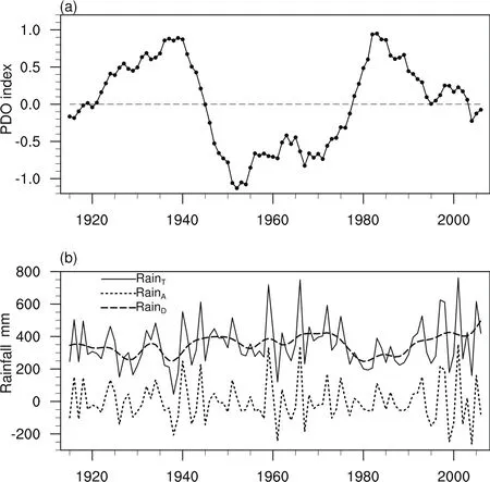
Fig.2.(a)The standardized time series of wintertime(October–March)PDO index and their 11-year running mean during 1915–2006.As an example,the year 1915 denotes October–December 1914 and January–March 1915.(b)Total rainfall(RainT,units:mm)in June during 1915–2006,which is decomposed into an interannual component(RainA)with variation less than 11 years and an interdecadal component(RainD)with variation longer than 11 years.

Figure 3 shows a schematic plot of the TSDTR approach to forecasting the SCESR based on the PLS regression method.On the interannual timescale,in order to incorporate the modulation e ff ect of the PDO on the interannual variability of SCESR(Mao et al.,2011;Duan et al.,2013), a threshold PLS regression model is calibrated for the relationship between RainAand SSTAunder the positive and negative phase of the PDO.On the interdecadal timescale, a standard PLS regression model is calibrated for the relationship between RainDand associated SSTDpatterns.The total rainfall prediction is obtained by the sum of the outputsfrom both the IAM and IDM(Fig.3). To test the performance of the TSDTR approach in forecasting the SCESR,the study period 1915–2006(N=92)is separated into a calibration period[1915–84(n=70)]and validation period(1985–2006).The two PLS-based regression downscaling models in the TSDTR approach are calibrated by using the calibration data in 1915–84,and the forecasting skill of the TSDTR is tested by the independent validation data in 1985–2006.To obtain the forecasted values in the independent validation period,we use the running forecasting method based on the calibrated models.That is,fort=n+1，n+2，...，N(=92),when the observed preceding SST(t)data and wintertime PDO are available over the validationperiod1985–2006,weaddthesenewSSTdatatothose in thetrainingperiod,andthen decomposethecombinedSST data into interannual SSTA(t)and interdecadal SSTD(t)components.The forecasted value of interannual[interdecadal] rainfall can be estimated by using SSTA(t)[SSTD(t)]and the calibrated IAM[IDM].The performance of the TSDTR downscaling approach is assessed through the correlation coefficient(CC)between predicted and observed values and the RMSE(Zhanget al.,2011;Guo et al.,2012).Theuncertainty oftheforecastis indicatedbythespreadofbootstrappingprediction intervals[see appendix in Liand Smith(2009)].

4. Forecasting SCESR

This section provides details of the TSDTR downscaling approach to building the IAM and IDM based on the PLS regression for the relationship between the preceding month SST and the SCESR on the interannual and interdecadal timescales,respectively.

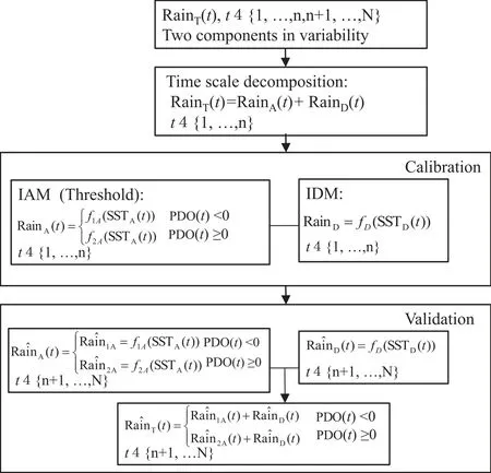
Fig.3.Schematic plot of the TSDTR approach to forecasting the SCESR.

4.1. Calibrating the IAM

The interannual variation of SCESR is remarkably different under diff erent PDO phases.Chan and Zhou(2005) demonstrated that the interannual relationship between ENSO and SCESR is modulated by the phase of the PDO. Mao et al.(2011)indicated that the interannual SCESR variations are remarkably diff erent under diff erent PDO phases, based on a comparison in two typical epochs of 1958–76 and 1980–98.Furthermore,it was suggested by Duan et al. (2013)that the predictability of interannual SCESR variability is modulated by diff erent PDO-phase backgrounds,and they also indicated that the relationship between interannual rainfall and preceding Pacific SST anomalies experienced a robust interdecadal change due to the PDO’s modulation through the so-called“seasonal footprinting mechanism”.

To further explore the predictability of interannual SCESR variability modulated by diff erent PDO-phase backgrounds,Fig.4 shows the lag-correlation patterns of interannual SCESR with precedinginterannualmonthly(May,April and March)SSTAover the Pacific and Indian oceans in negative and positive phases of the PDO,denoted by PDO(-) and PDO(+),respectively.It is evident that the interannual relationship between RainAand SSTAexhibits very diff erent structures during the positive and negative PDO phases.A striking diff erence in Fig.4 is that there is a traditional eastern Pacific warming ENSO-like correlation pattern between RainAand SSTAduring the PDO(+)phase,but a central Pacific warming ENSO-like pattern is more pronounced during the PDO(-)phase.Such correlation patterns may lead the SCESR by up to 3 months from March to May.This result is consistent with the result of Duan et al.(2013),who compared 1955–76 PDO(-)and 1977–98 PDO(+).The result supports the fact that the interannual SCESR variability and its relationshipwith ENSO are modulatedby the PDO phases (Chan and Zhou,2005;Zhou et al.,2006;Mao et al.,2011). Therefore,the interannual relationship between large-scale SST anomalies and the SCESR is not stationary due to the modulation of the PDO.As such,in order to incorporate the modulatione ff ectof thePDO ontheinterannualvariabilityof SCESR,we need to consider the nonstationary relationship between RainAand SSTAin the Pacific and Indian oceans. To this end,a threshold PLS regression model(Fig.3)is employed to establish the relationship between RainAand the leading SSTAmodes,which best explain the co-variations of RainAand SSTAunder the PDO(-)and PDO(+),separately.After a series of tests using SSTApredictors in each precedingmonth,includingtheprecedingMay,April,March, February,January,December and November,it is found that SSTAconditions in the preceding March tend to yield the best results.Thus,we concentrate on reporting the dominant SSTAmodes in Marchoverthe Pacific and Indian oceansthat in fl uence RainA.

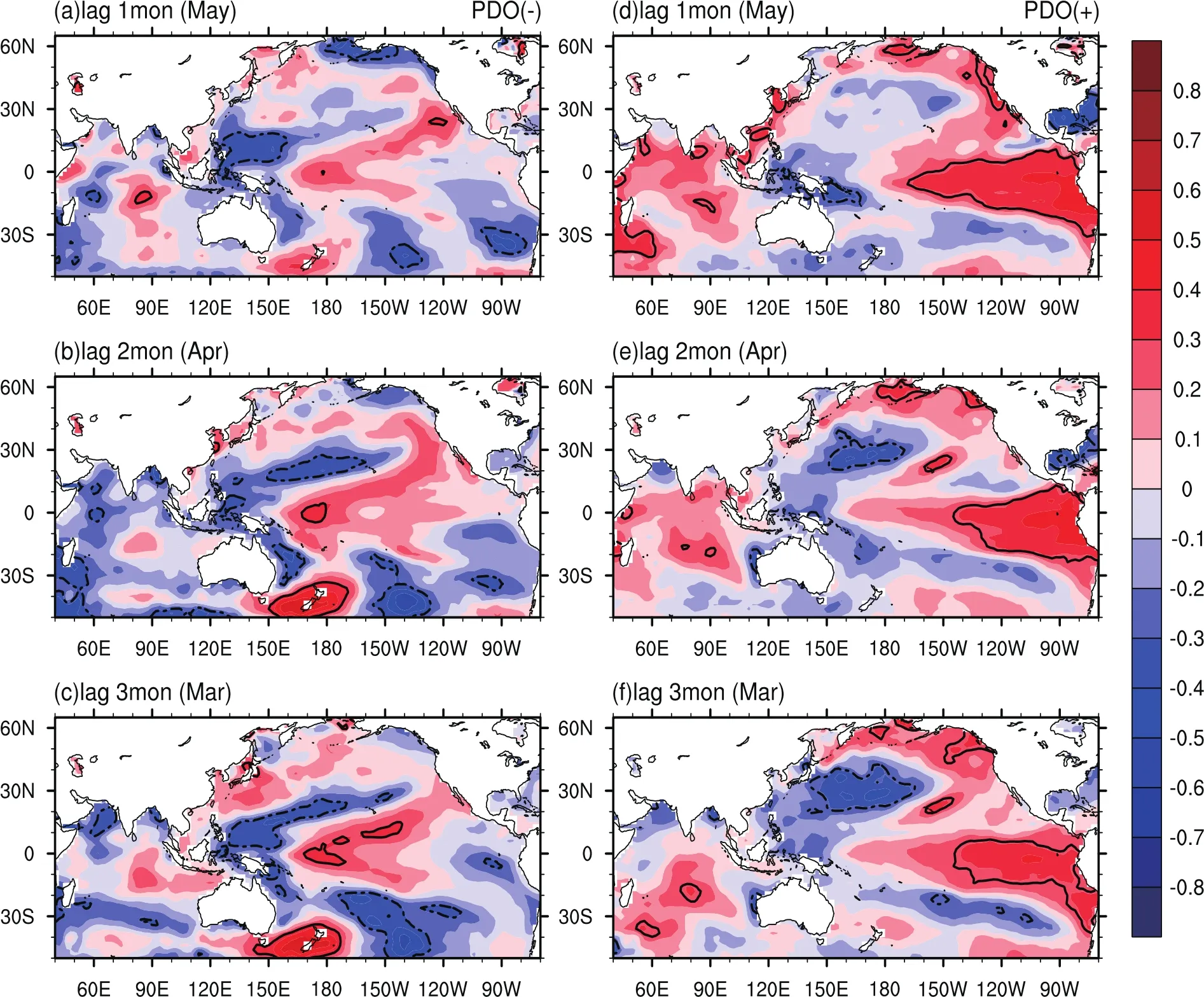
Fig.4.Lead–lag correlation of RainAwith SSTAin the Pacific and Indian oceans in the(a–c)negative phase and(d–f)positive phase of the PDO.The contour lines present the CCs of±0.3,statistically significant at the 95%con fidence level.

Figure 5 shows the first two leading interannual modes of March SST(SSTA-iand SSTA-II)represented by PLS loadings in PDO(-)and PDO(+),respectively.The significance of each mode is re fl ected by two numbers:the first is the percentage of RainAvariance explained by the SST-PLS mode; the other is the percentageof SSTAvariance explained by the sameSST-PLS mode.InPDO(-),the firsttwo leadingmodes together explain 73.2%of the total variance of RainA.The first dominant mode(Fig.5a)during the negative phase of the PDO is,by and large,an El Nin˜o Modoki–like pattern in the tropical Pacific region,with positive loadings in the central Pacific and negative loadings in the western and eastern Pacific.Another significant positive loading occurs over the South-central Pacific region around New Zealand.The tropical Indian Ocean is characterized by weak positive loadings. As shown in Fig.6a with respect to the corresponding patterns of precipitation and vertically integrated moisture fl ux to the SSTA-imode,notable southwesterly moisture transportation to the SC region is observed in the troposphere, which is accompanied by a significant low-level anomalous anticyclone located in the South China Sea and Philippine Sea(not shown).At the same time,southward penetration of northerly moisture transportation from a large part of North and Northeast China also exists and leads to significant moisture convergence over the SC region.Therefore,abundant interannual rainfall is received in this region(Fig.6a).

The second dominant SST mode(Fig.5b)in PDO(-)has strongnegativeloadingsin the central-easterntropicalPacific and weaker negative loadings in the tropical Indian Ocean, indicating a La Ni˜na–like pattern.Signals can also be found in the midlatitudes,with anomalous warming in the North Pacific region and South-central Pacific region around New Zealand.ThepatterninthetropicalandmidlatitudeNorthPacific resembles the anomalous SST features of negative PDO phase.Correspondingly,one can see notable southerly moisture transportation over the majority of eastern China(Fig. 6b),which is accompanied by an anomalous low-level anticyclonelocated in the north to northeast of the Philippine Sea (not shown).The SC region is under the control of southerly moisture transport,but the moist fl ows are strong enough to advance more northward.Thus,distribution of anomalous precipitation in China shows weak above-normalinterannual rainfall over SC(Fig.6b).

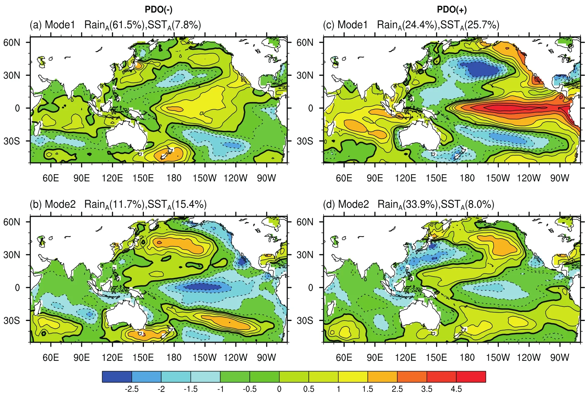
Fig.5.First two leading modes of March SSTAin the Pacific and Indian oceans from PLS regression analyses in the(a,b)negative phase and(c,d)positive phase of the PDO.The first percentage value is the total variance of RainAexplained by the SSTAmode, and the second value is the total SSTAvariance explained by the same mode.

In PDO(+),the first two leading modes together explain 58.3%of the total variance of interannual rainfall.The leading interannual SST modes(SSTA-iand SSTA-II)dramatically change in contrast with those in PDO(-).The first dominant mode(Fig.5c)tends to suggest a strengthened traditional El Ni˜no–like signal in in fl uencing the interannual early summer rainfall over SC during the positive phase of the PDO,with very strong positive loadings in the tropical eastern Pacific.Another positive loading occurs in the tropical Indian Ocean.In addition,the positive loading in the South-central Pacific region around New Zealand in PDO(-) is replaced by negative loading.Meanwhile,the pattern in themidlatitudeNorthPacificsharessimilarfeatureswithSST anomalies during the positive phase of the PDO.The circulation responses to this mode(Fig.6c)show notable southwesterly moisture transportation from the South China Sea to the southeast coast of China,which leads to above-normal precipitation over the SC region.The second dominant interannualSST mode(SSTA-II)inPDO(+)hasnegativeloadings in the central-eastern tropical Pacific that display a La Ni˜na–like pattern(Fig.5d),but has reduced in this mode compared with that in PDO(-)(Fig.5b).The Indian Ocean is occupied by weak negative loadings.In addition,a warming anomaly occurs in Peru’s inshore waters.Figure 6d shows the corresponding interannual circulation responses.The vertically integrated moisture fl ux pattern indicates that the main moisture source region for interannual rainfall over SC in this mode is from the Bay of Bengal.Through the westerly fl ows carrying warm and wet air,the SC region tends to receive above-normalinterannual rainfall.

Based onthe aboveanalysis,the diff erentleadinginterannual SST modes relatedto the interannualearly summerrainfall over SC in PDO(-)and PDO(+)may indicate that different PDO“backgrounds”modulatethe connectionbetween the interannual early summer SC rainfall and SST anomalies over the Pacific and Indian oceans.Therefore,when building a statistical forecasting model for interannual rainfall with preceding SST conditions,one needs to consider such nonlinearity.As previously mentioned,a threshold PLS regression model(Fig.3)is employed to establish the relationship between RainAand the leading SSTAmodes by taking into account the modulation of PDO(-)and PDO(+).

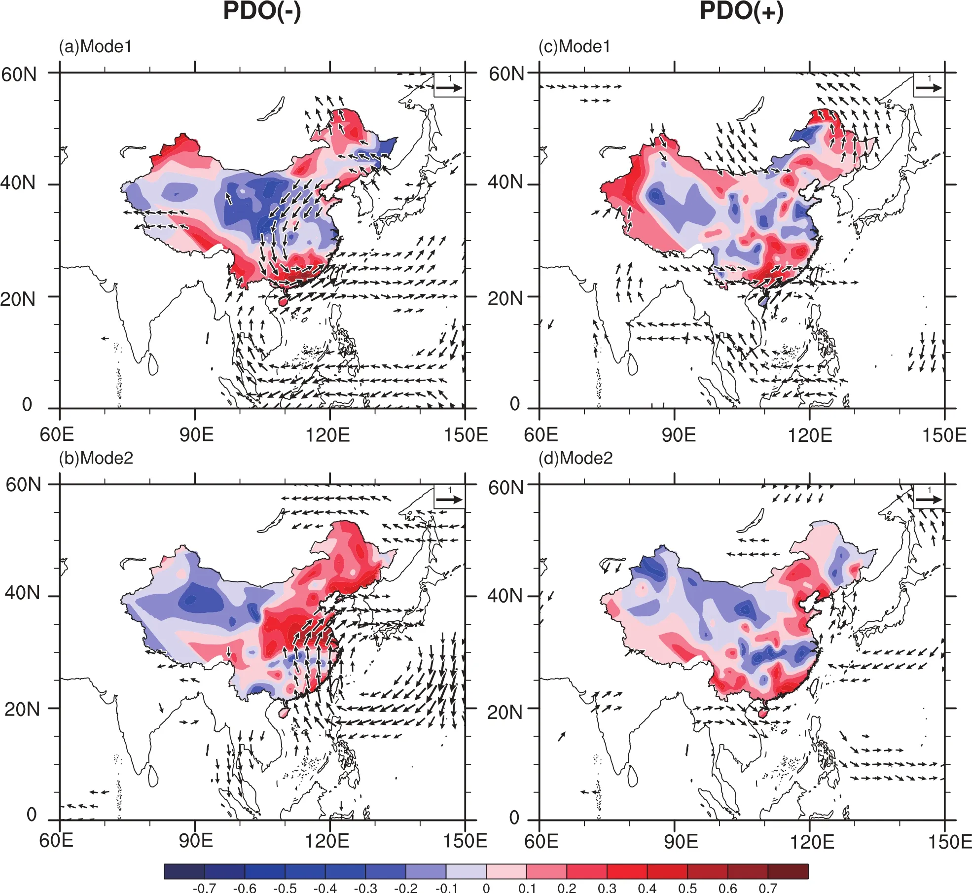
Fig.6.Correlations of the detrended scores of March SSTAmodes in Fig.5 with high-pass filtered June precipitation(color shading) and vertically integrated moisture fl ux between 1000 hPa and 300 hPa(vectors)in the(a,b)negative phase and(c,d)positive phase of the PDO.

Figure 7a compares the interannual variation of predicted and observed RainAvalues from the threshold PLS regression model(i.e.the IAM in Fig.3)based on the first two leading interannual SST modes,which is derived using observed data over the training periodof 1915–84(n=70).The results indicate that RainAcan be reconstructed with significant skill for the training period(Fig.7a),with a CC0of 0.87 and RMSE0of 54.45mm between the predicted and observed RainAvalues(Model IV in Table 1).Here,CC0and RMSE0are the CC and RMSE between the observed rainfall and reconstructed rainfall in the calibration period.To obtain the forecastedvalues[ˆRainA(t)]in the independentvalidation period of 1985–2006,we use the running forecasting method based on the calibrated IAM.The forecasted value of interannual rainfall[ˆRainA(t)]can be estimated by using SSTA(t) and the calibrated IAM(i.e.the calibrated threshold PLS regression model based on the preceding wintertime PDO phases).Figure 7a shows the forecasted values[ˆRainA(t)] in the validation period of 1985–2006 and their uncertainty in terms of bootstrapping 95%con fidence intervals.

4.2. Calibrating the IDM

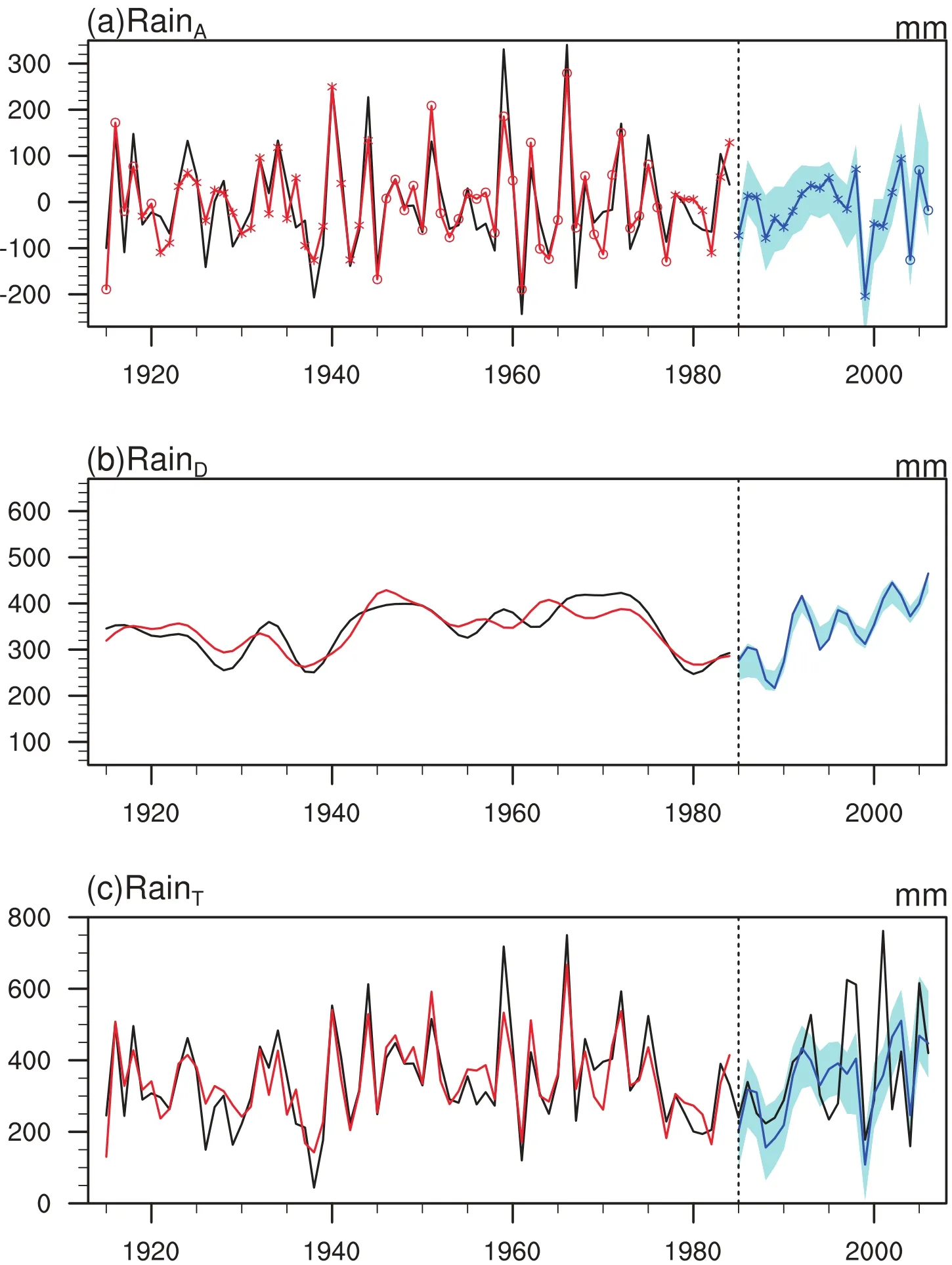
Fig.7.(a)PLS regression model results for forecasting RainA.PDO negative(positive)years are marked with“o”(“*”).The black line is the time series of observed RainA;the red line is the reconstructed RainAduring 1915–84;and the blue line is the hindcasted RainAduring 1985–2006.(b) PLS regression model results for forecasting RainD.The black line is the time series of observed RainD;the red line is the reconstructed RainDduring 1915–84;and the blue line is the hindcasted RainDduring 1985–2006.(c)Model results for forecasting the total rainfall.The black line is the time series of observed RainT;the red line is the reconstructed RainTduring 1915–84;and the blue line is the hindcasted RainTduring 1985–2006.The blue shading in each of the panels represents the upper and lower bands of the bootstrapping 95%con fidence intervals for the hindcasted values.

Next we develop an IDM for the interdecadal variability of the SCESR.Previous studies have noted that temporal variations of the SCESR exhibit an interdecadal oscillation related to the PDO,with more dry(wet)years during periods of positive(negative)PDO index(Chan and Zhou,2005; Duanet al.,2013).ChanandZhou(2005)alsomentionedthat the e ff ect of the PDO is more important than that of ENSO in the control of SCESR,although such a conclusion might be premature given our limited understanding of the PDO and ENSO,as well as their possible interaction.Because the rainfall and PDO index have a close negative relationship on the interdecadal timescale,and the most visible climatic fingerprints of the PDO exist in the North Pacific(Mantua et al.,1997;Mantua and Hare,2002),it is supposed that the most important interdecadal SST signal in fl uencing the interdecadal rainfall variability may exist in the midlatitude North Pacific region.With the aim to develop a PLS-based regression downscaling model with preceding interdecadal SST conditions to forecast the interdecadal rainfall variability,a series of tests using SSTApredictors in each preceding month,includingthe precedingMay,April,March,February, January,December and November,are conducted,and the results show that interdecadal SST conditions over the midlatitude western-central North Pacific[(20°–50°N,120°E–140°W)]in the preceding November give the best results. Thus,we focus on reporting the leading interdecadal SST modes in November over the western-central Pacific regionand the corresponding atmospheric circulation responses to the SST modes in fl uencing the interdecadal SC rainfall variability.To this end,the PLS regression model(Fig.3)is employed to establish the relationship between RainDand the leading SSTDmodes using the training data in the period 1915–84.

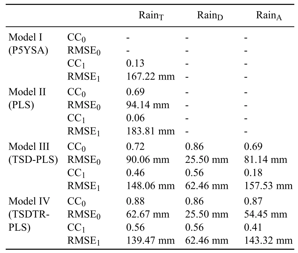
Table 1.Comparison of results from our rainfall forecasting model (Model I–IV)experiments.CC0and RMSE0(CC1and RMSE1)are the CC and RMSE between the observed rainfall and reconstructed (predicted)rainfall in the calibration(validation)period.

Figure 8 shows the first two leading interdecadal SST modes(SSTD-iand SSTD-II)represented by PLS loadings. These two leading modes together explain 74.1%of the variance of RainD,with the majority contributed from the first leading mode(58.1%).The SSTD-imode(Fig.8a)is characterized by significant positive loadings that almost cover the entire western-central North Pacific,with two maximum anomalousSST centers located in the Yellow Sea and midlatitude central North Pacific located at about(35°N,160°W). However,these positiveloadingsin thewestern-centralNorth Pacific shrink in the second mode(SSTD-II);instead,negative loadings widely expand(Fig.8b).The SSTD-imode resembles the characteristics of the PDO negative phase to some extent,with a typical warm SST anomaly pattern in the central North Pacific(Mantua et al.,1997;Mantua and Hare, 2002).This is therefore consistent with previous results in which persistent wet conditions overthe SC are related to periods of negative PDO index(Chan and Zhou,2005;Zhou et al.,2006).In the second dominant SST mode(SSTD-II),the shrinkingof positive loadings may imply a phase transformation from negative to positive PDO.

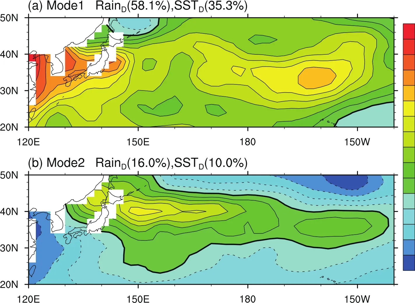
Fig.8.First two leading modes of November SSTDin the western-central North Pacific from PLS regression analyses.The first percentage value is the total variance of RainDexplained by the SSTDmode and the second number is the total SSTDvariance explained by the same mode.

To examine the corresponding atmospheric circulation anomalies associated with the above two dominant SST modes on the interdecadal timescale,we show the correlation patterns of the scores of SST modes with the vertically integrated moisture fl ux between 1000 hPa and 300 hPa(Fig. 9).The anomalous precipitation distributions in China are also displayed in Fig.9.For the SSTD-imode,remarkable southwesterly moisture fl ux enters into the SC region,whichwould lead to persistently wet conditions in the region(Fig. 9a).As a result,a significant positive correlation with interdecadal rainfall variability over the SC region ultimately occurs(Fig.9a).The atmospheric circulation responses to the second mode(SSTD-II)are basically similar to those for the first mode,only with small diff erences in magnitude,thus also exerting a bene ficial in fl uence on above-normal interdecadal rainfall variability over the SC region(Fig.9b).The SST anomalies in the North Pacific associated with the PDO can persist for 20–30 years,from winter to summer(Mantua et al.,1997),and thus seem to be important in the control of the persistently wet or dry conditionsin earlysummer over SC.Notethatsincetheanomaliesassociatedwithpersistently wetanddryconditionsgenerallytendto haveoppositepolarities,the reverse is true for interdecadal below-normal rainfall variability.

Figure 7b compares the interdecadal variation of predicted and observed RainDvalues from the PLS regression model(i.e.the IDM in Fig.3)based on the first two leading modes(SSTD-iand SSTD-II),which is derived using observed data over the training period of 1915–84(n=70).It is evident that the IDM can reproduce the time series of interdecadal rainfall variability in the training period well,with a CC0of 0.88 and RMSE0of 62.67 mm between the predicted and observed values of RainD.To obtain the forecasted interdecadal values[ˆRainD(t)]in the independent validation period of 1985–2006,we use the running forecasting method based on the calibrated IDM.The forecasted value of interdecadalrainfall[ˆRainD(t)]canbe estimated by usingSSTD(t) and the calibrated IDM.Figure 7b shows the forecasted values[ˆRainD(t)]inthevalidationperiodof1985–2006andtheir uncertainty in terms of bootstrapping 95%con fidence intervals.

4.3. Forecasting the SCESR

It is straightforward to forecast the values of the SCESR (i.e.RainT)by summing up the forecasted valuesˆRainA(t) andˆRainD(t)fromtheIAMandIDMmodels(i.e.the TSDTR downscaling approach).Figure 7c shows the performance of forecasting the SCESR.In general,the performance in the training period is maintained in the subsequent validation period.For example,compared to the observed climatological rainfall of 343.80 mm during the training period of 1915–84 and 367.70 mm during the validation period of 1985–2006, the statistical model provides a preproduction of 343.80 mm and 351.15 mm,respectively.The TSDTR downscaling approach provides reasonable forecasting skill by using preceding SST as the only predictor.Table 1 shows the forecasting skill of total rainfall by showing the associated CC (CC0=0.88)and RMSE(RMSE0=62.67 mm)between the downscaled and observed rainfall for the training period of 1915–84.This skill is maintained reasonably well in the validation period with a CC1of 0.56 and RMSE1of 139.47 mm (Table 1,Model IV).Here,CC1and RMSE1are the CC and RMSE between the observed rainfall and predicted rainfall in the validation period.The bootstrapping 95%con fidence intervals associated with the forecasted values are shown inFig.7c,indicating the uncertainty of the TSDTR downscaling approach.All these results indicate that the TSDTR downscaling approach can achieve some reasonable rainfall forecasting skill over SC.

Fig.9.Correlations of the detrended scores of November SSTDmodes in Fig.8 with low-pass filtered June precipitation(color shaded)and vertically integrated moisture fl ux between 1000 hPa and 300 hPa(vectors).

To see how well the TSDTR downscaling approach performs in forecasting the SCESR,compared to other simple methods,we examine three diff erent methods for forecasting the SCESR.We analyze the use of the previous 5 years′SCESR average(P5YSA),a single PLS model,and a TSDPLS model.The P5YSA is a computationally convenient and frequently used technique to forecast a regular time series,which is carried out without recourse to a formal statistical model.The single PLS model is calibrated by directly regressing the SCESR onto the SST field,while the TSD-PLS model is calibrated by two steps;namely,decomposing the rainfall and SST field into interannual and interdecadal components,and then applying the PLS method to them.All these three methods do not integrate the modulation of the PDO on the interannual relationship between SCESR and SST.Note that the first two dominant SST patterns are used in both the PLS and TSD-PLS models for a fair comparison with the TSDTR downscaling approach.Table 1 summarizes how the forecasting skill of the TSDTR downscaling approach compares with the three simpler models.The CC between the forecasted and observed SCESR values in the validation period for P5YSA,PLS and TSD-PLS are CC1=0.13,0.06 and 0.46,respectively,which is smaller than that(0.56)from the TSDTR downscaling approach.In addition,the RMSE between the forecasted and observed SCESR values in the validation period for P5YSA, PLS and TSD-PLS are RMSE1=167.22,183.81 and 148.06 mm,respectively—larger than the RMSE(RMSE1=139.47 mm)for the TSDTR downscaling approach.Therefore,the more complex TSDTR downscaling approach performs better than the simpler P5YSA,PLS and TSD-PLS models in forecasting the SCESR.We thus emphasize that the application of the newly proposed TSDTR method can improve regional rainfall prediction skill by incorporating the PDO modulatione ff ect,even when the skill of the pure PLS model is low.

In summary,the rationale behind the TSDTR downscaling approach is that it allows a model parameter change for the unstable relationship between the interannual rainfall variability and preceding SST conditions in diff erent PDO phases.As a result,the TSDTR downscaling approach can further improve rainfall forecasting skill by considering the modulation e ff ect of decadal-scale coupled oceanic–atmospheric modes on interannual climate variability,compared to other simpler methods(e.g.P5YSA,PLS and TSDPLS),without considering the preceding SST conditions in diff erent PDO phases.

5. Summary and discussion

This paper puts forward the TSDTR downscaling approach to forecast SCESR by using preceding SST over the Indian and Pacific oceans through modeling the interannual and interdecadal rainfall variability via an IAM and IDM. The IAM is built upon a threshold PLS regression by taking account of the modulation e ff ect of the PDO on the interannual variability of the SCESR.Through the IAM,the first two leading March SST modes(an El Ni˜no Modoki–likepattern and a La Ni˜na–like pattern)are linked to the interannual rainfall in the negative phase of the PDO,while the first two leading modes(a strengthened traditional El Ni˜no–like pattern and a La Ni˜na–like pattern)are linked to the interannual variability of the SCESR in the positive phase of the PDO. The first two leading interdecadal SST modes are linked to the interdecadalcomponentof the SCESR via the IDM based on the PLS regression method.The forecasted total rainfall is obtained by summing up the values of the two forecasted components from the IAM and IDM.

In applying the TSDTR approach to forecasting SCESR, it is found that the interannual relationship between the preceding Pacific–Indian Ocean SST and SCESR experiences interdecadal changes,displaying remarkable diff erences in the negativeand positivephases of the PDO.In particular,the traditional ENSO-like anomalous SST pattern is robust only in the PDO positive phase.For interdecadal rainfall variability,the dominant interdecadal SST patterns over the North Pacific resemble some characteristics of the PDO.When the North Pacific SST is persistently warming(cooling),the interdecadal variability of SCESR tends to be below-normal (above-normal).This is consistent with previous studies in which persistentlywet(dry)conditionsoverSC in early summer are related to periods of negative(positive)PDO index (Chan and Zhou,2005;Duan et al.,2013).

A central implication of this study is that regional rainfall forecasting skill can be improved via the TSDTR approach,wherein the unstable relationship between interannual rainfall and large-scale variability,such as SST,can be taken into the process of model development.For a statistical downscalingmodel,it is important to select the predictors that have the most stable relationships with observed rainfall(Sun and Chen,2012):If the predictor has a stable relationship with the predictand,the predictability of the statistical downscaling scheme developed using this predictor will be stable;otherwise,a predictor with an unstable relationship with the predictand could result in unstable predictability of the statistical downscaling scheme.As the TSDTR approach considers the modulation e ff ect of decadal-scale coupled oceanic–atmosphericmodeson interannualclimate variability,it may provide a new perspective to improve climate prediction.In this paper,we demonstrate that the TSDTR downscaling forecasting skill is superior to three other simpler methods(P5YSA,PLS and TSD-PLS),without considering the preceding SST conditions in diff erent PDO phases. The results suggest that the TSDTR approach has a higher predictive capability SCESR.

In spite of the improvement in forecasting skill,the TSDTR downscaling forecasting model for SCESR encounters a problemin that it fails to predictsomeextreme fl oodevents, such as in 2001.This failure is attributable to the interannual rainfall model,because the preceding interannual spring SST condition used as the predictor in 2001 displays no significant anomalies(not shown),indicating that the SST anomaly itself is not the only factor that can exert an important in fl uence on the interannualSC rainfall.Thus,research gaps exist insofar as other potential factors need to be considered in the development of the TSDTR model.We expect in the future to include some of these other factors[e.g.the atmospheric circulation variability over the extratropics and tropics,and soil moisture conditions(e.g.Thompson and Wallace,1998; Zhao et al.,2007;Chen et al.,2014)],with theaim to improve the statistical forecasting skill further.

Acknowledgements.This workwassponsoredbytheNational Basic Research Program of China(Grant No.2012CB955202). Linye SONG received support from the China Scholarship Council under the Joint-PhD program for conducting research at CSIRO. Yun Liwas supported by the Indian Ocean Climate Initiative.

Appendix A PLS regression

PLS regression is usually described as a two-staged approach.Following Butler and Denham(2000),the first stage is to produce a sequence of k≤m PLS components Zioflengthnto be included in the regression.However,unlike principal components,which are only formed by accounting for the maximum amount of joint variability ofXXX,the PLS componentZi(i=1，2，...，k)is chosen to explain as much as possible the covariance betweenXXXandY.That is,

where εkis the appropriate error term.The parameterbiis derived by minimizing the sum of squares,

Note that the selectedZi(i=1，2，...，k)is obtained by accountingfor the maximumamountof the covariancebetweenXXXandY.Thus,PLS componentsare obtained by not only accounting for the variance of explanatoryvariablesXXX,but also the variances in the predicantY.

REFERENCES

Aligo,E.A.,W.A.Gallus Jr.,and M.Segal,2009:On the impact of WRF model vertical grid resolution on Midwest summer rainfall forecasts.Wea.Forecasting,24,575–594.

Butler,N.A.,and M.C.Denham,2000:The peculiar shrinkage properties of partial least squares regression.Journal of the Royal Statistical Society:Series B(Statistical Methodology),62,585–593.

Cao,X.,S.F.Chen,G.H.Chen,W.Chen,and R.G.Wu,2015:On the weakened relationship between spring Arctic Oscillation and following summer tropical cyclone frequency over the western north Pacific:A comparison between 1968-1986 and 1989-2007.Adv.Atmos.Sci.,32,1319–1328,doi:10.1007/ s00376-015-4256-y.

Cao,X.,S.F.Chen,G.H.Chen,and R.G.Wu,2016:Intensified impact of northern tropical Atlantic SST on tropical cyclogenesis frequency over the western North Pacific after the late 1980s.Adv.Atmos.Sci.,doi:10.1007/s00376-016-5206-z.

Chan,J.C.L.,and W.Zhou,2005:PDO,ENSO andthe earlysummer monsoon rainfall over south China.Geophys.Res.Lett.,32,L08810.

Chen,S.-F.,W.Chen,B.Yu,and H.-F.Graf,2013a:Modulation of the seasonal footprinting mechanism by the boreal spring Arctic Oscillation.Geophys.Res.Lett.,40,6384–6389,doi: 10.1002/2013GL058628.

Chen,S.F.,B.Yu,and W.Chen,2014:An analysis on the physical process of the in fl uence of AO on ENSO.Climate Dyn.,42, 973–989.

Chen,S.F.,B.Yu,and W.Chen,2015a:An interdecadal change in the in fl uence of the spring Arctic Oscillation on the subsequent ENSO around the early 1970s.Climate Dyn.,44,1109–1126.

Chen,S.F.,W.Chen,and R.G.Wu,2015b:An interdecadal change in therelationship between boreal spring ArcticOscillation and the East Asian Summer Monsoon around the early 1970s.J.Climate,28,1527–1542.

Chen,W.,J.Feng,and R.G.Wu,2013b:Roles of ENSO and PDO in the link of the East Asian Winter Monsoon to the following Summer Monsoon.J.Climate,26,622–635.

Collischonn,W.,R.Haas,I.Andreolli,and C.E.M.Tucci,2005: Forecasting River Uruguay fl ow using rainfall forecasts from a regional weather-prediction model.J.Hydrol.,305,87–98.

Ding,Y.H.,Z.Y.Wang,and Y.Sun,2008:Inter-decadal variation of the summer precipitation in East China and its association withdecreasing Asian summer monsoon.Part I:Observed evidences.Int.J.Climatol.,28,1139–1161.

Duan,W.S.,L.Y.Song,Y.Li,and J.Y.Mao,2013:Modulation of PDO on the predictability of the interannual variability of early summer rainfall over south China.J.Geophys.Res.,118,13 008–13 021.

Eitzen,Z.A.,and D.A.Randall,1999:Sensitivityof thesimulated Asian summer monsoon to parameterized physical processes.J.Geophys.Res.,104,12 177–12 191.

Gao,H.,Y.G.Wang,and J.H.He,2006:Weakening significance of ENSO as a predictor of summer precipitation in China.Geophys.Res.Lett.,33(9),L09807,doi:10.1029/2005 GL025511.

Gershunov,A.,and T.P.Barnett,1998:Interdecadal modulation of ENSO teleconnections.Bull.Amer.Meteor.Soc.,79,2715–2726.

Gong,D.-Y.,and C.-H.Ho,2002:Shift in the summer rainfall over the Yangtze River valley in the late 1970s.Geophys.Res. Lett.,29,78-1–78-4.

Grotch,S.L.,and M.C.MacCracken,1991:The use of general circulation models to predict regional climatic change.J.Climate,4,286–303.

Guo,Y.,J.P.Li,and Y.Li,2012:A time-scale decomposition approach to statistically downscale summer rainfall over North China.J.Climate,25,572–591.

Haenlein,M.,and A.M.Kaplan,2004:A beginner’s guide to partial least squares analysis.Understanding Statistics,3,283–297.

Helland,I.S.,1988:On the structure of partial least squares regression.Communications in Statistics-Simulation and Computation,17,581–607.

Huang,R.H.,and Y.F.Wu,1989:The in fl uence of ENSO on the summer climate change in China and its mechanism.Adv. Atmos.Sci.,6,21–32,doi:10.1007/BF02656915.

Huang,R.H.,J.L.Chen,G.Huang,and Q.L.Zhang,2006: The quasi-biennial oscillation of summer monsoon rainfallin China and its cause.Chinese Journal of Atmospheric Sciences,30,545–560.(in Chinese)

Kalnay,E.,and Coauthors,1996:The NCEP/NCAR 40-year reanalysis project.Bull.Amer.Meteor.Soc.,77,437–472,doi: 10.1175/1520-0477(1996)077＜0437:TNYRP＞2.0.CO;2.

Lau,K.M.,and H.Y.Weng,2001:Coherent modes of global SST and summer rainfall over China:An assessment of the regional impacts of the 1997-98 El Ni˜no.J.Climate,14,1294–1308.

Li,Y.,and I.Smith,2009:A statistical downscaling model for southern Australia winter rainfall.J.Climate,22,1142–1158.

Liu,Y.,and K.Fan,2012a:Improve the prediction of summer precipitation in the Southeastern China by a hybrid statistical downscaling model.Meteor.Atmos.Phys.,117,121–134.

Liu,Y.,and K.Fan,2012b:Prediction of spring precipitation in China using a downscaling approach.Meteor.Atmos.Phys., 118:79–93.

Liu,Y.,and K.Fan.2014:An application of hybrid downscaling model to forecast summer precipitation at stations in China.Atmospheric Research,143:17–30.

Mantua,N.J.,and S.R.Hare,2002:The Pacific decadal oscillation.Journal of Oceanography,58,35–44.

Mantua,N.J.,S.R.Hare,Y.Zhang,J.M.Wallace,and R.C. Francis,1997:A Pacific interdecadal climate oscillation with impacts on salmon production.Bull.Amer.Meteor.Soc.,78, 1069–1079.

Mao,J.Y.,J.C.L.Chan,and G.X.Wu,2011:Interannual variations of early summer monsoon rainfall over South China under diff erent PDO backgrounds.Int.J.Climatol.,31,847–862.

Martin,G.M.,1999:The simulation of the Asian summer monsoon,and its sensitivity to horizontal resolution,in the UK meteorological office unified model.Quart.J.Roy.Meteor. Soc.,125,1499–1525.

Nitta,T.,and Z.-Z.Hu,1996:Summer climate variability in China and its association with 500 hPa height and tropical convection.J.Meteor.Soc.Japan Ser.II,74,425–445.

Power,S.,T.Casey,C.Folland,A.Colman,and V.Mehta,1999: Inter-decadal modulationof theimpact of ENSOonAustralia.Climate Dyn.,15,319–324.

Sahai,A.K.,A.M.Grimm,V.Satyan,and G.B.Pant,2003:Longlead prediction of Indian summer monsoon rainfall from global SST evolution.Climate Dyn.,20,855–863.

Smith,T.M.,and R.W.Reynolds,2004:Improved extended reconstruction of SST(1854-1997).J.Climate,17,2466–2477.

Smith,T.M.,R.W.Reynolds,T.C.Peterson,and J.Lawrimore,2008:Improvements to NOAA’s historical merged land-ocean surface temperature analysis(1880–2006).J.Climate,21,2283–2296.

Smoliak,B.V.,J.M.Wallace,M.T.Stoelinga,and T.P.Mitchell, 2010:Application of partial least squares regression to the diagnosis of year-to-year variations in Pacific Northwest snowpack and Atlantic hurricanes.Geophys.Res.Lett.,37, L03801,doi:10.1029/2009GL041478.

Sun,J.Q.,and H.J.Wang,2012:Changes of the connection between the summer North Atlantic Oscillation and the East Asian summer rainfall.J.Geophys.Res.,117,D08110,doi: 10.1029/2012JD017482.

Sun,J.Q.,and H.P.Chen,2012:A statistical downscaling scheme to improve global precipitation forecasting.Meteor.Atmos. Phys.,117,87–102.

Tao,S.Y.,1987:A review of recent research on the East Asian summer monsoon in China.J.Meteor.Soc.Japan,70,373–396.

Thompson,D.W.J.,and J.M.Wallace,1998:The Arctic oscillation signature in the wintertime geopotential height and temperature fields.Geophys.Res.Lett.,25,1297–1300.

Torrence C.,and P.J.Webster,1999:Interdecadal changes in the ENSO-monsoon system.J.Climate,12,2679–2690.

Wang,B.,LinHo,Y.S.Zhang,and M.M.Lu,2004:De finition of South China Sea monsoon onset and commencement of the East Asia summer monsoon.J.Climate,17,699–710.

Wang,B.,R.G.Wu,and X.Fu,2000:Pacific-east Asian teleconnection:How does ENSO a ff ect east Asian climate?J. Climate,13,1517–1536.

Wang,H.J.,2001:The weakening of the Asian monsoon circulation after the end of 1970’s.Adv.Atmos.Sci.,18(3),376–386, doi:10.1007/BF02919316.

Wang,H.J.,2002:The instability of the East Asian summer monsoon-ENSO relations.Adv.Atmos.Sci.,19(1),1–11,doi: 10.1007/s00376-002-0029-5.

Wang,L.,W.Chen,R.H.Huang,2008:Interdecadal modulation of PDO on theimpact of ENSOon theeast Asian winter monsoon.Geophys.Res.Lett.,35,L20702,doi:10.1029/2008 GL035287.

Wilby,R.L.,1998:Statistical downscaling of daily precipitation using daily air fl ow and seasonal teleconnection indices.Climate Research,10,163–178.

Wu,R.G.,and B.Wang,2002:A contrast of the East Asian summermonsoon-ENSO relationshipbetween1962-77 and1978-93.J.Climate,15,3266–3279.

Wu,R.G.,S.Yang,Z.P.Wen,G.Huang,and K.M.Hu,2012:Interdecadal change in the relationship of southern China summer rainfall with tropical Indo-Pacific SST.Theor.Appl.Climatol.,108,119–133.

Wu,Z.W.,H.Lin,Y.Li,and Y.M.Tang,2013:Seasonal prediction of killing-frost frequency in South-Central Canada during the cool/overwintering-crop growing season.Journal of Applied Meteorology and Climatology,52,102–113.

Zhang,H.Q.,J.Qin,and Y.Li,2011:Climatic background of cold and wet winter in southern China:part iobservational analysis.Climate Dyn.,37,2335–2354.

Zhao,P.,Z.J.Zhou,and J.P.Liu,2007:Variability of Tibetan spring snow and its associations with the hemispheric extratropical circulation and East Asian summer monsoon rainfall: An observational investigation.J.Climate,20,3942–3955.

Zhou,W.,C.Li,and J.C.L.Chan,2006:The interdecadal variations of the summer monsoon rainfall over South China.Meteor.Atmos.Phys.,93,165–175.

Zhu,C.-W.,C.-K.Park,W.-S.Lee,and W.-T.Yun,2008:Statistical downscaling for multi-model ensemble prediction of summer monsoon rainfall in the Asia-Pacific region using geopotential height field.Adv.Atmos.Sci.,25,867–884,doi: 10.1007/s00376-008-0867-x.

:Song,L.Y.,W.S.Duan,Y.Li,and J.Y.Mao,2016:A timescale decomposed threshold regression downscaling approach to forecasting South China early summer rainfall.Adv.Atmos.Sci.,33(9),1071–1084,

10.1007/s00376-016-5251-7.

∗Corresponding author:Wansuo DUAN

Email:duanws@lasg.iap.ac.cn