Several Nonconvex Models for Image Deblurring under Poisson Noise∗

LIU Gang,HUANG Ting-zhu

(School of Mathematical Sciences,University of Electronic Science and Technology of China,Chengdu 611731)

1 Introduction

Image deblurring under Poisson noise is a fundamental problem in image processing,which plays a critical role in a wide range of applications,and positron emission tomography(PET),see[1–6]and references therein.Without loss of generality,we only consider the square image with the size of n×n for simplicity,and all our results can be easily extended to general rectangular images with the size of m×n,because we deal with an image by pulling the columns of the two-dimensional matrix into a vector.Let f∈Rn2be the original image and g be the observed image corrupted by Poisson noise.Diff erent from the additive Gaussian white noise[7],the degradation process of Poisson noise is that each pixel of the observed image is modeled as an independent random variable under Poisson distribution whose expectation equals to the value of the corresponding pixel in the original image.In detail,according to the Poisson distribution,we have the following conditional probability distribution

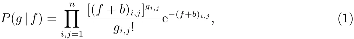
where b is a background parameter which is assumed to be known,fi,jrefers to the((j−1)n+i)th entry of the vector f,it is the(i,j)-th pixel location of the n×n image,and this notation remains valid throughout the paper unless otherwise specified.

The estimation of the original image f from the observed image g is an inverse problem which is typically ill-posed[8].The Poisson noise degradation process limits the direct applications of the traditional least square fi delity term for Gaussian noise removal[9].In[10,11],the authors proposed some advanced regularization models for Poisson noise removal derived from a maximum a posteriori(MAP)framework.MAP is actually the same as maximizing the function P(g|f)by minimizing the negative logarithm of the likelihood function.After some calculations,one obtain the Kullback-Leibler divergence[8]

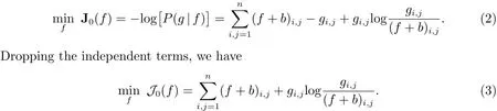
It is easy to show that the function J0(f)is proper[10,12,13]and convex[11].In particular,if gi,j>0 for some(i,j),J0(f)is strictly convex.The function J0(f)usually serves as the fi delity term in the Poisson noise removal model for measuring the closeness of the solution to the observed data.

During acquisition and transmission,Poisson images are often degraded by blur[14].We assume the blur matrix(denoted as H)is known,then the fidelity term for image deblurring under Poisson noise reads

If the blurring marix H is nonsingular,then the fi delity term in(4)is strictly convex.However,due to the ill-condition of H,the minimizer of problem(4)does not lead to a satisfactory solution.To obtain reliable results,a popular and eff ective strategy is to add to(4)a regularization term J(f),also known as a priori knowledge of the original image[15].

One of popular regularization terms is the total variation(TV)regularization term[10,16],and it can preserve imageedges well.In recent years,extensiveoptimization methods have been increasingly applied for solving TV based models;see,e.g.,[17–25].The original TV model in[16]is given in an isotropic form(ITV),and later on it is extended to an anisotropic variant(ATV)in[26].The mathematical defi nitions for both ITV and ATV in the discrete setting are given respectively as follows

Here,|·|denotes the pointwise absolute value and ∇ :Rn2→ Rn2denotes the discrete gradient operator(under periodic boundary conditions):

More details for the defi nition of the TV regularization can be found in[27,28].

Let Dxand Dybe the matrices generated by the diff erence operator∇xand∇y,respectively.Let Df=(Dxf,Dyf),then

In the literature of sparse representation,researchers reconstruct signals from under-determined systems by assuming that the signal is suffi ciently sparse or sparse in a transformed domain,for instancethewavelet transform[29,30].From thispoint of view,TV can be considered as imposing sparsity in the gradient domain[31,32].Mathematically,it amounts to minimizing the L0norm,J(f)= ∥Df∥0.To bypass the NP-hard of L0,the convex relaxation approach is used to replace L0by L1,which is actually the TV regularization.In order to guarantee the equivalence of L1and L0,theoretical results require the restricted isometry property(RIP)condition[33].However,the RIP condition often does not hold for image deblurring and denoising.Therefore,for better approximation of L0,several nonconvex penalties have been proposed and studied as variants of L1,such as Lp(p∈(0,1))[34],L1−L2[35,36].To the best of our knowledge,these nonconvex regularization terms are only considered to removal Gaussian noise and has not been applied to Poisson image restoration.

In this paper,we extend the existing nonconvex regularizers Lpand L1−L2to Poisson image restoration.First,we propose two models with weighted diff erence of convex(DC).One is L1− αL2,the other is L1− αLOGSbased on the recent OGS regularizer[37-39].For these two DC models,we provide effi cient numerical algorithms and establish theconvergenceresultsbased on thesuccessiveupper-bound minimization(SUM)in[40].Second,we propose an L2/3model based on the results in[34].For this model,we develop an algorithm based on the symmetric alternating direction method of multipliers(SADMM)[41-43].Although the convergence of SADMM for nonconvex problemsisstill open,our numerical schemeishighly effi cient becauseof theclosed-form solution[34]of each subproblem involved,which isalso verifi ed by numerical experiments.Numerical results show that theproposed models achieve an enhanced gradient sparsity and yield restoration results competitive with some existing methods.

The outline of this paper is as follows.In section 2,we give the formulations of the proposed models as well as numerical algorithms.The numerical results are given in section 3.Finally,we conclude this paper in section 4.

2 Three nonconvex models and their solving algorithms

First,to better understand the metrics of the nonconvex functions,we plot the 2-dimensional surfaces corresponding to L1−L2,L1−0.5L2,L1−0.5LOGSand L2/3in comparison with L0and L1in Figure 1.For the L0norm,the value is zero at origin,1 at axes,and 2 elsewhere.From the figure,we know that L2/3is most closed to L0,and that L1−0.5L2is better than L1−L2.All nonconvex metrics are more closed to L0than L1.In our numerical experiments,we will fi nd that our models are competitive with the L1based model and promote sparsity.

2.1 Two DC models and their algorithms

According to the above discussions,we propose our fi rst DC model,the L1−αL2model(Model 1),by combining the fi delity term and the regularization term

The second DC model is the L1−αLOGSmodel(Model 2)shown as follows

Given a vector v∈Rn2(relevant matrix or image V ∈Rn×n),let

⌊y⌋denotes the largest integer less than or equal to y.vi,j,K1,K2is the relevant vector of the matrix Vi,j,K1,K2,and then

More details about LOGScan be found in[37–39].

Figure 1:2-dimensional surfaces of diff erent metrics.From left top to right bottom,L 0,L 1,L 1−L 2,L 1−0.5L 2,L 1−0.5L OGS and L 2/3

It isnot easy to solvetheabovetwo DC modelsdirectly.Based on SUM[40],weneed to fi nd the majorizers of the two functions.For simplicity,we only give the details for Model 1,and then similarly for Model 2.First,we use a linear function to approximate the L2norm as follows

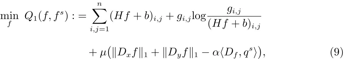
where⟨x,y⟩denotes the inner product(which isx y),and

ii

In the next section,we will show that Q1(f,fs)is a majorizer of P1(f)and that the sequence{fs}converges to the stationary point of P1(f).Here,we focus on the inner convex subproblem argmfin Q1(f,fs).We use the SADMM method[41-43]to solve it.SADMM is a variation of the classic ADMM,and its convergence speed is much faster than the classic ADMM[43].Moreover,we also consider the box constraint[0,255]on pixel values(similar work can be found in[44]).Then,we have

In details,the constraint reads

Then,the SADMM scheme for prlblem(11)is

where f[k]denotes the k th iteration of SADMM which is diff erent from outer iterations fsin(10).SADMM always converges to one of the global minimizers for convex models[43].However,the object function of(11)is not always strong convex,so the solution isoften not unique.Thus we choose two suitable positiveparametersβ1,β2>0 to make the SADMM algorithm converges to our expected minimizer.

In(12),for the A subproblem,variables(z,y1,y2,w)aredecoupled and then can be solved separately.For the f subproblem,it is a least square problem,which is easy to solve by a normal equation.With fast Fourier transforms(FFTs),this normal equation can be solved fast and easily[14,17].Therefore,all the former subproblems can be solved easily,and then the algorithm of Model 1 is provided.The algorithm for Model 2 is very similar to that for Model 1,thus we omit the details.

Clearly,for the y1subproblem(y2is similar)

Theminimization with respect to y1can begiven explicitly by thewell-known Shrinkage method[45].

where sgn and “◦” represent the signum function and the componentwise product,respectively.

For the z subproblem

Note that the minimization in problem(15)is separable with respect to each component.The solution of problem(15)is

For the w subproblem

For the f subproblem

The minimizer can be obtained by equivalently solving the following normal equation

2.2 Convergence analysis

In this section,we will show that the sequence{fs}obtained from the proposed algorithm,i.e.(10),converges to a stationary point.

Lemma 1 Supposeµ>0,0<α<1,Model 1 and Model 2 are proper,continuous and coercive.Then the minimizers exist.

Proof We only prove the coercive property of Model 1.Obviously,we have

The final part P1,0of the last equation(just as the TV Poisson deblurring)is coercive by[10].Therefore,when∥f∥→∞,P1,0→∞,and then P1→∞.The proof is complete.

In particular,ifα=0,our Model 1 degenerates to the classic ATV model(L1norm).Ifα<0,our Model 1 is a sum of two convex function and also convex,this is not the scope of this paper.

Lemma 2 For all f,fs,we have

Proof In fact,since ∥Df∥2,1− ⟨Df,qs⟩is convex on f,then we can get the minimum is0.After simple calculation,wehave−∥Df∥2,1≤ −⟨Df,qs⟩.Then,P1(f)≤Q1(f,fs).In addition,it is easy to know P1(f)=Q1(f,f).

Therefore,we have

The second inequality comes from the generation of fs+1.

Theorem 1 Under the assumptions in Lemma 1,any non-zero limit point of{fs}generated by(10)is a stationary point of P1(f).

Assume that there exists a subsequence{fsj}coverging to a limit point u,then we have

which implies(f,u;d)|f=u≥ 0, ∀ d.Therefore,we obtain(u;d)≥ 0, ∀ d,which implies that u is a stationary point of P1(f).

On the other hand,it is easy to show that Q1(f,fs)is coercive on f.According to the generation of each fs+1,we know that the sequence{fs}is bounded.Then,the convergent subsequence of the sequence{fs}exists.The proof is now completed.

2.3 The L 2/3 model and its solution algorithm

Our third nonconvex model is the Lpmodel with 0

It is very similar to(11),except the y1,y2subproblems.When p=1/2,2/3,these two subproblems have closed-form solutions from[34],and we choose p=2/3 in this paper since the results in[34]are better than those for p=1/2.That is,we only need to change the yisubproblems(13)of(11)according to the closed-form solution in[34].Although the convergence of SADMM for nonconvex problems is still open,our numerical scheme is highly effi cient because of the closed-form solution[34]of each subproblem involved,which is also verified by numerical experiments.We do not consider other p∈(0,1)because they do not have closed-form solutions.

3 Numerical exp eriments

Thequality of therestoration resultsismeasured quantitatively by using thesignalto-noiseratio(SNR)in decibel(d B)and thestructural similarity index(SSIM)[46].The SNR is defi ned as

whereand f denote the original and restored images,respectively,f¯ denotes the mean of the original imagefˆ.

As for SSIM,the reader can refer to[46]for more details.We only use it as a black box to measure the quality of the restoration images.The closer to 1 the SSIM is,the better the result is.

We compare our methods with some other existing methods.One is the classic ATV method(L1)as in[25],and another method is the L0norm as in[31,47,48].In Model 1 and Model 2,we setα=1/2 based on the discussion in[36].We set the first outer iteration f1=g,the observed image.

The original images are shown in Figure 2:2015,House,Lena,Peppers.The original images are blurred by three blur kernels:

(i) Gaussian blur 5-by-5 with standard deviation 1(“G” for short);

(ii) Motion blur 5-by-5 with angle of 45 degrees(“M” for short);

(iii) Average blur 3-by-3(“A” for short).

Then,they are corrupted by Poisson noise.The background parameter b is set to 10.The maximum value of the original image is fi xed at 255.For other parameters,we tune them based on the highest SSIM.

Figure 2:Original images,from left to right,2015,House,Lena,Peppers

The numerical results of the diff erent methods are shown in Table 1.The last three columns correspond to our methods,and “Bn”denotes blurred and noisy images.From thetable,wecan find that our nonconvex models arecompetitivewith theexiting methods,such as L0and L1methods.From[49],we know that the SSIM is more important than SNR,so we illuminate the SSIM more clearly.And through this,the advantages of our methods are highlighted.From Table 1,we can see that occasionally the results of our nonconvex models are worse than L1,but at lease one of the proposed models is better than L1.

Moreover,wedisplay thedegraded imagesand restored imagesin Figure3 to Figure 6.Not only do the proposed models work well on horizonal or vertical edges by design,they can deal with natural images as well.From the figures,we can see the visual improvement is similar to those numerical advantages in Table 1.

Table 1:Numerical comparisons for diff erent methods on SNR(d B)and SSIM(×10−4)

Figure 3:Results of image“2015” under Average blur.From left top to right bottom,blurred and noisy image,the results of L 0,L 1,L 1−0.5L 2,L 1−L OGS and L 2/3

Figure 4:Results of image “House” under Gaussian blur.From left top to right bottom,blurred and noisy image,the results of L 0,L 1,L 1−0.5L 2,L 1−L OGS and L 2/3

Figure 5:Results of image “Lena” under Motion blur.From left top to right bottom,blurred and noisy image,the results of L 0,L 1,L 1−0.5L 2,L 1−L OGS and L 2/3

Figure 6:Results of image “Peppers” under Gaussian blur.From left top to right bottom,blurred and noisy image,the results of L 0,L 1,L 1−0.5L 2,L 1−L OGS and L 2/3

Next,for our Model 1 and Model 2,we will show that the outer iteration s is often selected by 2 or 3 which is suffi cient.It means that in many cases,we can use a linear function to approximate the L2norm,and the results are much close to the original results.

In addition,we plot the function values and relative errors against the iterations in Figure 7 for Model 1 and Model 2 on image“Lena” under Gaussian blur.The function values are P1(f)for L1−0.5L2and P2(f)for L1−0.5LOGS.The relative errors are the relative errors of f between two inner iterations.From the figure,and after similar tests on other images and blurs,we fi nd that our two DC methods only need 1 to 3 outer iterations to get good results.Moreover,we can see that our algorithms for two DC models converge.Occasionally,in the inner iterations,we find that the function values may not decrease.It is because the inner convex approximate functions are diff erent from the original nonconvex functions,while the function values in the figure are the original functions.The same situation occurs for the relative errors.However,the function values of each fi nal inner iteration(the outer iteration function values)decrease,which verifies the theoretical convergence result.Moreover,from the figure,wealso see that sometimes a good convex approximate model may have a high accuracy of the original nonconvex model.For instance,in this example,only one outer iteration is enough.

Figure 7:Function values and relative errors against the iterations of L 1−0.5L 2,L 1−0.5L OG S on image “Lena” under Gaussian blur.From left to right,function values against iterations of L 1−0.5L 2,relative errors against iterations of L 1−0.5L 2,function values against iterations of L 1−0.5L OGS,relative errors against iterations of L 1−0.5L OGS

Sparsity In addition,we examine the sparsity of the gradient vectors Df.Defi ne a gradient vector of a pixel as non-sparse if both Dxf and Dyf at that pixel are larger than 1.5(every pixel in[0,255]).Then,we can calculate the percentage of nonsparse gradient vectors over the total number of pixels.The sparsity percentage of the examples is presented in Table 2,here we only list the results for Figure 3 to Figure 6.From the table,we can see that,all our methods promote sparsity through producing the more sparse gradients than L1and L0.This is the motivation of our nonconvex models.Sometimes,L2/3is the best,and sometimes our three methods are close to each other.The poor performance of L0is because that L0is not easy to solve and the numerical method is not best.

Table 2:The percentages(%)of non-sparse gradient vectors Df of the results obtained with L 0,L 1,L 1−0.5L 2,L 1−0.5L OGS and L 2/3 regularization terms in comparison to Df of the original image

4 Conclusion

In thispaper,weproposed several nonconvex modelsand developed thecorresponding solution algorithms.For the two DC models,we found good convex approximate models to solve them.Under the SUM algorithm frame,wetheoretically prove that the algorithms converge to the stationary points,which is a typical situation for nonconvex problems.For the L2/3model,wedeveloped an algorithm based on SADMM.Moreover,according to the numerical tests,the proposed models achieved an enhanced gradient sparsity and yielded restoration results competitive with some existing methods.

References:

[1]Dupe F X,Fadili J M,Starck J L.A proximal iteration for deconvolving Poisson noisy images using sparse representations[J].IEEE Transactions on Image Processing,2009,18(2):310-321

[2]Zanella R,Boccacci P,Zanni L,et al.Effi cient gradient projection methods for edge-preserving removal of Poisson noise[J].Inverse Problems,2009,25(4):045010

[3]Keenan M R,Kotula P G.Accounting for Poisson noise in the multivariate analysis of ToF-SIMS spectrum images[J].Surface and Interface Analysis,2004,36(3):203-212

[4]Bertero M,Boccacci P,Talenti G,et al.A discrepancy principle for Poisson data[J].Inverse Problems,2010,26(10):105004

[5]Staglian´o A,Boccacci P,Bertero M.Analysis of an approximate model for Poisson data reconstruction and a related discrepancy principle[J].Inverse Problems,2011,27(12):125003

[6]Le T,Chartrand R,Asaki T J.A variational approach to reconstructing images corrupted by Poisson noise[J].Journal of Mathematical Imaging and Vision,2007,27(3):257-263

[7]Gonzalez R C,Woods R E.Digital Image Processing[M].USA:Prentice Hall Inc,2006

[8]Csiszar I.Why least squares and maximum entropy?An axiomatic approach to inference for linear inverse problems[J].The Annals of Statistics,1991,19(4):2032-2066

[9]Vio R,Bardslev J,Wamsteker W.Least-squares methods with Poissonian noise:analysis and comparison with the Richardson-Lucy algorithm[J].Astronomy&Astrophysics,2005,436(2):741-755

[10]Bardsley J M,Luttman A.Total variation-penalized Poisson likelihood estimation for ill-posed problems[J].Advances in Computational Mathematics,2009,31(1-3):35-59

[11]Chen D Q,Cheng L Z.Spatially adapted regularization parameter selection based on the local discrepancy function for Poissonian image deblurring[J].Inverse Problems,2012,28(1):015004

[12]Bertsekas D P,Nedic A.Convex Analysis and Optimization[M].Belmont:Athena Scientifi c,2003

[13]Bonnans J F,Gilbert J C,Lemarbbchal C,et al.Numerical Optimization:Theoretical and Practical Aspects[M].Berlin Heidelberg:Springer,2006

[14]Hansen P C,Nagy J G,O’Leary D P.Deblurring Images:Matrices,Spectra,and Filtering[M].Philadelphia:Society for Industrial and Applied Mathematics,2006

[15]Bertero M,Boccacci P,Desider`a G,et al.Image deblurring with Poisson data:from cells to galaxies[J].Inverse Problems,2009,25(12):123006

[16]Rudin L I,Osher S,Fatemi E.Nonlinear total variation based noise removal algorithms[J].Physica D,1992,60(1-4):259-268

[17]Wang Y L,Yang J F,Yin W T,et al.A new alternating minimization algorithm for total variation image reconstruction[J].SIAM Journal on Imaging Sciences,2008,1(3):248-272

[18]Yang J F,Yin W T,Zhang Y,et al.A fast algorithm for edge-preserving variational multichannel image restoration[J].SIAM Journal on Imaging Sciences,2009,2(2):569-592

[19]Esser E.Applications of Lagrangian-based alternating direction methods and connections to split Bregman[R].UCLA CAM Report,2009:9-31

[20]Eckstein J,Bertsekas D P.On the Douglas-Rachford splitting method and the proximal point algorithm for maximal monotone operators[J].Mathematical Programming,1992,55(1-3):293-318

[21]Wu C L,Tai X C.Augmented Lagrangian method,dual methods,and split Bregman iteration for ROF,vectorial TV,and high order models[J].SIAM Journal on Imaging Sciences,2010,3(3):300-339

[22]Goldstein T,O’Donoghue B,Setzer S,et al.Fast alternating direction optimization methods[J].SIAM Journal on Imaging Sciences,2014,7(3):1588-1623

[23]Chan T F,Golub G H,Mulet P.A nonlinear primal-dual method for total variation-based image restoration[J].SIAM Journal on Scientifi c Computing,1999,20(6):1964-1977

[24]Cai J F,Osher S,Shen Z W.Split Bregman methods and frame based image restoration[J].Multiscale Modeling and Simulation,2010,8(2):337-369

[25]Figueiredo M A T,Bioucas-Dias J M.Restoration of Poissonian images using alternating direction optimization[J].IEEE Transactions on Image Processing,2010,19(12):3133-3145

[26]Esedo¯glu S,Osher S J.Decomposition of images by the anisotropic Rudin-Osher-Fatemi model[J].Communications on Pure and Applied Mathematics,2004,57(12):1609-1626

[27]Chambolle A.An algorithm for total variation minimization and applications[J].Journal of Mathematical Imaging and Vision,2004,20(1-2):89-97

[28]Guo X X,Li F,Ng M K.A fastℓ1-TV algorithm for image restoration[J].SIAM Journal on Scientifi c Computing,2009,31(3):2322-2341

[29]Figueiredo M A T,Nowak R D.An EM algorithm for wavelet-based image restoration[J].IEEE Transactions on Image Processing,2003,12(8):906-916

[30]Chai A,Shen Z.Deconvolution:a wavelet frame approach[J].Numerische Mathematik,2007,106(4):529-587

[31]Xu L,Lu C W,Xu Y,et al.Image smoothing via L0gradient minimization[J].ACM Transactions on Graphics,2011,30(6):1-12

[32]Asif M S,Romberg J.Fast and accurate algorithms for re-weightedℓ1-norm minimization[J].IEEE Transactions on Signal Processing,2013,61(23):5905-5916

[33]Cand`es E J,Romberq J K,Tao T.Stable signal recovery from incomplete and inaccurate measurements[J].Communications on Pure and Applied Mathematics,2006,59(8):1207-1223

[34]Cao W F,Sun J,Xu Z B.Fast image deconvolution using closed-form thresholding formulas of Lq(q=)regularization[J].Journal of Visual Communication and Image Representation,2013,24(1):31-41

[35]Yin P H,Lou Y F,He Q,et al.Minimization ofℓ1−2for compressed sensing[J].SIAM Journal on Scientifi c Computing,2015,37(1):A536-A563

[36]Lou Y F,Zeng T Y,Osher S,et al.A weighted diff erence of anisotropic and isotropic total variation model for image processing[J].SIAM Journal on Imaging Sciences,2015,8(3):1798-1823

[37]Liu G,Huang T Z,Liu J,et al.Total variation with overlapping group sparsity for image deblurring under impulse noise[J].PloS One,2015,10(4):e0122562

[38]Liu J,Huang T Z,Selesnick I W,et al.Image restoration using total variation with overlapping group sparsity[J].Information Sciences,2015,295(20):232-246

[39]Liu G,Huang T Z,Lv X G,et al.New explicit thresholding/shrinkage formulas for one class of regularization problems with overlapping group sparsity and their applications[OL].E-print,http://ar Xiv.org/abs/1312.6813,2013

[40]Razaviyayn M,Hong M,Luo Z Q.A unifi ed convergence analysis of block successive minimization methods for nonsmooth optimization[J].SIAM Journal on Optimization,2013,23(2):1126-1153

[41]Glowinski R.Numerical Methods for Nonlinear Variational Problems[M].Berlin Heidelberg:Springer,1984

[42]Glowinski R,et al.On the convergence of operator-splitting methods[C]//Kuznetsov P,et al.,Numerical Methods for Scientifi c Computing,Variational Problems and Applications,2003:67-79

[43]He B S,Liu H,Wang Z R,et al.A strictly contractive peaceman–rachford splitting method for convex programming[J].SIAM Journal on Optimization,2014,24(3):1011-1040

[44]Chan R H,Tao M,Yuan X M.Constrained total variation deblurring models and fast algorithms based on alternating direction method of multipliers[J].SIAM Journal on Imaging Sciences,2013,6(1):680-697

[45]Yang J F,Zhang Y,Yin W T.An effi cient TVL1 algorithm for deblurring multichannel images corrupted by impulsive noise[J].SIAM Journal on Scientifi c Computing,2009,31(4):2842-2865

[46]Wang Z,Bovik A C,Sheikh H R,et al.Image quality assessment:from error visibility to structural similarity[J].IEEE Transactions on Image Processing,2004,13(4):600-612

[47]Blumensath T,Yaghoobi M,Davies M E.Iterative hard thresholding and L0regularisation[C]//IEEE International Conference on Acoustics,Speech and Signal Processing(ICASSP),Honolulu,HI:IEEE,2007:877-880

[48]Yan M.Restoration of images corrupted by impulse noise and mixed Gaussian impulse noise using blind inpainting[J].SIAM Journal on Imaging Sciences,2013,6(3):1227-1245

[49]Wang Z,Bovik A C.Mean squared error:love it or leave it?A new look at signal fi delity measures[J].IEEE Signal Processing Magazine,2009,26(1):98-117