Fault detection for nonlinear discrete-time system s via deterministic learning

Junmin HU,Cong WANG,Xunde DONG

School of Automation Science and Engineering,South China University of Technology,Guangzhou Guangdong 510640,China;Guangdong Key Laboratory of Biomedical Engineering,Guangzhou Guangdong 510640,China

1 Introduction

The design and analysis of fault detection and isolation(FDI)for nonlinear system s are important issues in modern engineering system s.In complex nonlinear system s,the faults are often hidden among the modeling uncertainties.For nonlinear system s with structured modeling uncertainties,in which the faults generated from nonlinear structure and cannot be decoupled from the unknown inputs.For diagnosis of non-linear system s with unstructured modeling uncertainties and nonlinear faults,the issue is much challenging since the faults cannot be decoupled from the unstructured modeling uncertainties.Over the past decades,much progress has been achieved for FDI of nonlinear continuous-time system s with structured and unstructured modeling uncertainties[1–14].In particular,adaptive threshold approaches using neural networks have recently received much attention for FDI of nonlinear system s with unstructured modeling uncertainties[10–14].However,only limited results has been obtained for fault diagnosis of nonlinear discrete-time system s[15–19].On the other hand,due to the increasing popularity of applying digital Computers in engineering,discrete-time system s can be more veritable to describe practical problem in control systems than continuous-time system s.The analysis and synthesis of fault detection(FD)for nonlinear discrete-time system s should be received m ore attention.Specifically,in[16],based on a parametric model of the faults,compensation of the fault effect on the state prediction is achieved via an adaptive discrete-time approach.A solution for fault isolation and identification is also proposed by using postfault analysis.In[18],an online approximation based fault detection and diagnosis scheme for multiple state or output faults was proposed for a class of nonlinear multiple-input-multiple-output(M IMO)discrete time system s.The faults considered could be incipient or abrupt,and were modeled using input and output signals of the system.In[19],a distributed fault detection and isolation approach based on adaptive approximation was proposed for nonlinear uncertain large-scale discrete-time systems.Local and global FDI schemes w ere provided due to the utilization of specialized fault isolation estimators and a global fault diagnoser.

In adaptive approximation based fault detection and isolation of general nonlinear system s,however,convergence of the em ployed neural network(NN)w eights to their optimal values and accurate neural network approximation of nonlinear fault functions were less investigated.Recently,a deterministic learning theory was proposed for identification,control and recognition of nonlinear dynamical system s exhibiting periodic or recurrent trajectories[20–22].By using localized RBF neural networks,it is shown that almost any periodic or recurrent trajectory can lead to the satisfaction of a partial persistent excitation(PE)condition,which in turn yields accurate neural network approximation of the system dynamics in a local region along the periodic or recurrent trajectory.Further,rapid recognition of a test dynamical pattern from a set of training dynamical patterns is achieved by using the locally accurate neural network approximation of system dynamics[21,22].Based on deterministic learning theory,in[23]a FD scheme was proposed for rapid detection of small oscillation faults generated from nonlinear continuous-time system s.The modeling uncertainty and nonlinear fault functions are firstly accurately approximated via deterministic learning,and then the know ledge is utilized to achieve rapid detection of small oscillation faults.

In this paper,a fault detection scheme is proposed for a class of nonlinear discrete-time system s based on deterministic learning theory.First,the internal dynamics underlying normal and fault m odes of nonlinear discrete-time system s are locally-accurately approximated by discrete-time dynamical RBF networks via a discrete-time extension of deterministic learning algorithm.Second,by utilizing the know ledge of system dynamics obtained through deterministic learning,a bank of estimators is constructed for the training normal and fault modes,and by com paring the set of estimators with the monitored system,a set of residuals are obtained and used to measure the differences between the dynamics of the monitored system and the dynamics of the trained systems.Finally,when the monitored system is in normal mode,the estimator corresponding to the normal mode will yield the smallest residual.When the monitored system is in one of the fault m odes,the residual of the fault estimator corresponding to this fault mode will become small and the residual of the normal estimator will become large.This means that the occurrence of a fault can be detected in a discrete-time setting according to the smallest residual principle.The fault detectability analysis is carried out and the upper bound of detection time is derived.Com pared with existing results on FD for nonlinear discrete-time systems,the main feature of this paper is that with locally-accurate approximation of the general fault functions of nonlinear discrete-time system s achieved via deterministic learning,the detection sensitivity to small faults of nonlinear discrete-time system s is increased substantially.

The rest of this paper is organized as follows.Section 2 begins with the introduction of deterministic learning theory,followed by the formulation of the problem in Section 3.In Section 4,the modeling and representation of the general fault function via deterministic learning for normal and fault modes is presented.On this basis,the detection scheme is given according to the smallest residual principle.Simulation results are included in Section 5.Section 6 concludes the paper.

2 deterministic learning theory

In this section,we briefly review deterministic learning theory,which is developed for NN identification,recognition and control of nonlinear dynamical system s undergoing periodic or recurrent trajectory[21,22].In deterministic learning theory,identification of system dynamics of general nonlinear systems is achieved according to the following elements:i)employment of localized RBF networks;ii)satisfaction of a partial PE condition;iii)exponential stability of the adaptive system along the periodic or recurrent orbit;and iv)locally-accurate NN approximation of the unknown system dynamics.

The presented deterministic learning theory,especially the approach for identification and rapid recognition of dynamical patterns,provides a solution for the problem of rapid detection and isolation of oscillation faults generated from uncertain nonlinear system s[22,23].The result may be further applied to the analysis of practical problem s.For instance,in[24],an approach for approximately accurate modeling and rapid detection of stall precursors based on deterministic learning and dynamical pattern recognition was developed.The studies on Mansoux model based on low speed axial compressor of Beihang University were conducted to show the effectiveness of the approach.Zeng and Wang[25,26]presented an algorithm to eliminate the effect of walking speed for efficient gait recognition in the lateral view.Then hum an gait dynamics underlying different individuals’gaits across different walking speeds were locally accurately approximated using deterministic learning.A method for electrocardiogram(ECG)pattern modeling and recognition via deterministic learning theory w as also presented in[27].

2.1 RBF network and PE condition

The RBF networks can be described by

whereZ∈ΩZ⊂Rqis the input vector withqbeing the NN input dimension,is the weight vector,Nis the NN node number,andwithsi(·)being a radial basis function,and ξi(i=1,...,N)being distinct points in state space.The Gaussian functionis one of the most comm only used RBF,whereis the center of the receptive field and ηiis the width of the receptive field.The Gaussian function belongs to the class of localized radial basis functions in the sense that

It has been shown in[20–22]that for any continuous functionwhere ΩZ⊂Rqis a com pact set,and for the NN approximator,where the node number N is sufficiently large,there exists an ideal constant weight vectorsuch that for eachwhere|є(Z)|＜ є＊is the approximation error.Moreover,for any bounded trajectoryZζ(t)within the com pact set ΩZ,f(Z)can be approximated by using a limited number of neurons located in a local region along the trajectory ϕζ:

wherewithNζ＜N,is a small positive constant,,and єζis the approximation error,withbeing small.

Based on previous results on the PE property of RBF networks[21],it is show n that for a localized RBF networkWTS(Z)w hose centers are placed on a regular lattice,almost any recurrent trajectoryZ(t)can lead to the satisfaction of the PE condition of the regressor sub-vectorSζ(Z)[22].

The following definition of persistency of excitation(PE)in discrete form provided by[28]is utilized.

Definition 1A sequenceS(k)∈Rnis said to be persistently exciting(inNsteps),if there existsN∈Z+,α＞0 such that

uniformly int0.

2.2 deterministic learning of discrete-time system s

The deterministic learning theory is extended to modeling and control of nonlinear discrete-time system s in[29–31].

A nonlinear discrete-time system in the following form is considered:

whereX=[x1···xn]T∈Rnis the state of the system,which is measurable,pis a system parameter vector,and differentpwill in general produce different dynami-cal patterns,is a smooth but unknown nonlinear vector field.

By using the following dynamical RBF network,spatially localized learning for discrete-time system s is achieved.

whereis the estimation of state vector,X(k)is the state of system(4),A=d iag{a1,...,an}is diagonal m atrix,is the design constant,andis a RBF networks used to approximate the unknown nonlinearityF(·;p)of(4),is the weight estimate,andis updated by

The identification scheme[22]describes a method of adjusting the NN weightsˆWin(6)in order to satisfy

A constant vector of neural weights is chosen as

with{ka,...,kb}representing a time segment after the transient process.We have that locally-accurate approximation of system dynamics along the tracking orbit ϕζcan be obtained as follows[22]:

w here ε＊is the ideal approximation error,ε1is the practical approximation error for using,and ε2is the practical approximation error for usingIn deterministic learning,both convergence of partial neural network weights to their optimal values and locally-accurate approximation of system dynamics can be achieved.This im plies that eitheris indeed capable of approximating the system dynamics to the desired error level ε＊,i.e.,ε1=O(ε＊)and ε2=O(ε1)=O(ε＊),which ensure that ε1and ε2are close to ε＊.

3 Problem formulation

Consider the following class of uncertain nonlinear discrete-time system:

whereis the state vector of the system,is the control input vector,kis the discrete-time instant.is unknown smooth nonlinear vector field representing the dynamics of the normal model,η(x(k),u(k))stands for the uncertainties including external disturbances,modeling errors and possibly discretization errors.The faultis the deviation in system dynamics due to faults(s=1,...,M),and β(k−k0)represents the fault time profile,withk0being the unknown fault occurrence time.Whenand w hen

The system state is assumed to be observable,and the system input is usually designed as a function of the system states.An assumption regarding the state and input of nonlinear discrete-time system is given as follow s.

Assumption 1The system statesx(k)are bounded for both normal and fault modes.

The state sequenceof(10)with initial conditionx(0)is defined as the system trajectory.The trajectory in normal mode is denoted as ϕ0(x(0))or ϕ0for conciseness of presentation,and the trajectory in fault modesis denoted as ϕs(x(0))or ϕsfor conciseness of presentation.

Assumption 2The system trajectories for both normal and fault modes are recurrent trajectories.

Rem ark 1A recurrent trajectory represents a large set of periodic and period-like trajectories generated from nonlinear dynamical system s,which includes periodic,quasi-periodic,almost-periodic,and even chaotic trajectories[32].Roughly speaking,a recurrent trajectory is characterized as follow s[33]:given a vector ς＞0,there exists aT(ς)＞0 such that the trajectory returns to the ς-neighborhood of any point on the trajectory within a time not greater thanT(ς).A remarkable feature of the recurrent trajectories is that,regard less of the choice of the initial condition,for any given ς-neighborhood the whole trajectory lies in the-neighborhood of the segment of the trajectory corresponding to a bounded time intervalT(ς).

Recurrent trajectories are comm on types of behaviors for nonlinear dynamical system s,which com prise the most important types(though not all types)of trajectories generated from nonlinear dynamical system s.Many practical dynamical system s,such as rotating machineries[34],electronic system s[35],power systems[36],[37],communication network[38],ECG system s[39],etc.,can exhibit such kind of trajectories or oscillations.Therefore,this approach can be widely applied in the practical system s.Moreover,deterministic learning theory has been applied to the practical rotating machinery[24],gait silhouettes[25]and ECG system s[27].

Rem ark 2In this paper,the system of fault detection is investigated with observable state.In practice,accurate measurement of all system states m ay not be available.Fault detection for the nonlinear system s with partial-state measurement can be studied by combining the approach proposed in this paper and the approach proposed in Chapter 7 of[22],in which deterministic learning algorithm s with partial-state measurement are presented.Due to the limitation of space,this issue will not be pursued in this paper.In the practical system s,which exhibit periodic or recurrent trajectories,the state vectors are bounded(or oscillatory).For example,the currents of power distribution system s are oscillating in the normal situation.When high impedance faults occur,the oscillations will be distorted but still remain lower than the over current thresholds[37].Such oscillating faults are similar to the normal behaviors and are very difficult to be detected.

In general,the uncertainties represented by the vector field η(x(k),u(k))is unstructured.For the design and analysis of a detection scheme,the following assumption is needed.

Assumption 3η(x(k),u(k))is bounded in a compact region by som e known functioni.e.

When the system is in fault m odes,since the fault functions may be hidden by the uncertainties,the uncertainties η(x(k),u(k))and the fault functions β(k−cannot be deco up led from each other.The two term s are considered together as an undivided term,and is defined as the general fault function[23]:

wheres=1,...,M,φs(x(k),u(k))represents thesth fault belongs to the set of fault functions.For simplicity of presentation,the normal mode is represented by fault modes=0,withi.e.,

For both normal and fault modes,combined with(11),system(10)can be represented by

wheres=0,1,...,M.

4 Fault detection for nonlinear discrete-time systems

4.1 Fault modeling and representation

Construct the follow ing discrete-time dynamical RBF network:

whereA=diag{a1,...,an}is a diagonal matrix,withbeing design constant,is the state vector of(13),is the state vector of system(10),is the prediction ofˆx(k).The Gaussian RBF networkis used to approximate the general fault function(11).

To ad just the NN w eightsˆW,the adaptive law(6)is designed as[30].

Rem ark 3The parameters of learning system,including the adaptive law(6),constant vector of neural weights(8)and dynamical RBF network(13),are set according to the analytic results proposed in[22],[30]and[40].For example,increasing the node number will decease the RBF approximation error,while the setting of the RBF widths will affect the level of persistent excitation,which in turn will also affect the learning capability of the proposed scheme.The observer gainaiis small,increasingaiwill increase the convergence rate of the estimated parameters.Whenaiincreases to a certain extent,increasingaiwill decrease convergence rate of the estimated parameters and deteriorates the ability of the dynamical RBF network(13)to learn the dynamics of the fault.Please see[40]for the detail discussion of the relationship betweenaiand the learning capability of the deterministic learning method.The way of setting Γiin the adaptive law(6)is similar to that of settingai.

Lemma 1Consider the close-loop system consisting of the nonlinear discrete-time system(12),the dynamical RBF network(13)and the NN update law(6).For both normal and fault modes of(12),we have that all the signals in the closed-loop system remain bounded,and the general fault function ψs(x(k),u(k))of system(12)is locally-accurately approximated along the trajectory ϕsbyas w ell as by(see(8)).

ProofThe proof of Lemma 1 can be found in[30].

Based on the convergence result ofˆW,w e can obtain a constant vector of neural weights¯Waccording to(8),such that

where є1and є2are the approximation errors usingandrespectively.It is clear that after the transient process,is small.In other word,the general fault functionof system(12)can be represented by using the constant RBF networkalong the trajectory ϕs(defined in Section 3).This representation,based on the fundamental information extracted from the trajectory ϕs,is independent of time[22].It w as also showed that the constant RBF networks¯W sTS(x(k))trained via deterministic learning naturally have a certain ability of generalization[22].

Rem ark 4In the literature of NN-based fault diagnosis,neural networks are used to provide powerful modeling tools.Nevertheless,for diagnosis of general nonlinear system s,it is very restrictive to verify a priori that the PE condition is satisfied[14].Consequently,it is difficult to guarantee that the employed neural networks can truly approximate the system dynamics and fault functions.In this paper,it was shown that both system dynamics for normal and fault m odes can be locally accurately approximated through deterministic learning.The sensitivity to small nonlinear faults is increased substantially,since the modeling uncertainties are reduced,and locally-accurate information of nonlinear faults is provided by using the constant NNs.

Note that the NN approximation of ψs(x(k),u(k))is accurate only in a local region along the trajectory ϕs.For the region far away from trajectory ϕs,the general fault function ψs(x(k),u(k))is not learned.This reveals that both the normal and fault m odes of nonlinear discrete time system s can be represented by using the locally accurate approximation of their underlying system dynamics along the state trajectories.The local region Ωϕsis described by[29]

whereis the approximation error within Ωϕs,dis a positive constant.The representation can be used in a way that whenever the NN input enters the region Ωϕsagain,the RBF networkwill provide accurate approximation to the dynamics ψs(x(k),u(k)).

Therefore,by learning the normal system and various fault system s,a bank of the trained system is represented by the corresponding constant RBF networks.

4.2 Fault detection

In this section,residuals generation and the fault decision scheme is presented,then a rigorous detectability analysis of the proposed detection scheme is also provided.

To be specific,the monitored system is described by

whererepresents the deviation of system dynamics due to an unknown fault.

For the monitored system(16),the general fault function is described by

By utilizing the learned know ledge about various trained system s,a dynamical model is constructed as follow s:

whereis the state of the dynamical model,is the state of monitored system(16),B=d iag{b1,...,bn}is a diagonal matrix which is kept the same for all normal and fault models,with 0＜bi＜1.is the learned know ledge of one trained system.

By combining the monitored system(16)and the dynamical model(18),the following residual system is obtained:

whereis the state estimation error(residual),andis the difference of system dynamics between the monitored system and thehth estimator.

The following averageL1norm of residuals is provided for making decision:

whereK∈Z+is the preset period constant of the monitored system.

Based on the above mentioned averageL1norm of residual,we have the following fault detection scheme for a class of nonlinear discrete-time system s.

Fault detection decision schemeCom parewith.If,fors∈{1,...,M},there exists some finite timeand somei∈{1,...,n}such thatthen the occurrence of a fault is deduced.

The absolute fault detection time instantKdis defined as the first time instant such thatfor someand som ei∈{1,...,n},that is,[14].The fault detection timekdis defined as the difference between the fault occurrence timek0and the absolute fault detection timeKd,i.e.,kd=Kd−k0[13,23].

Lemma 2Consider the monitored system(16),the fault estimator(18)and the residual system(19).For alls∈{1,...,M},i∈{1,...,n}andk∈[K,k0),when no fault occurs,if the following conditions hold:

1)there exists at least one intervalI=[ka,kb−1]⊆[k−K,k−1]such that

where

2)bisatisfies

Thenholds for allk∈[K,k0).for allk∈[K,k0).

For the monitored system(16),prior to the occurrence of faults,the general fault function is described by

Proof

In the time periodthe error dynamics with respect to the nominal model satisfies

The solution to the above equation is

From(15),we have

whereis given by(15).

By combining(26)and 0＜bi＜1,w e have

Sincexi(0)is available,we letthen,

Thereby,we have for allk≥K＞1,

The error dynamics with respect to thesth model satisfies

Thus,forkτ∈I,

From(15)and(21),we have

withandI′be defined as

Letl,l′denote the length of the time intervalIandI′respectively,thereby

The magnitude ofin the time intervalIcan be discussed in the following cases:

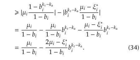
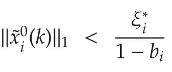
Consider(34),ifthen there exists a finite time instantsuch that

Solving the above inequality foryields

which im p lies that

From the above discussion,w e can summarize that there at most exists one time intervaland

Thus,in light of(20),we have for allk≥K＞1,

with(28)and 0＜bi＜1,(38)can be written as

The following theorem characterizes the fault detectability properties which include the fault detectability condition and detection time.

Theorem 1Consider the monitored system(16),the fault estimator(18)and the residual system(19).For somes∈{1,...,M},somei∈{1,...,n}andk≥k0+K,if the following conditions hold:

1)there exists at least one intervalI=[ka,kb−1]⊆[k−K,k−1]such that

where

2)bisatisfies

Then,

1)the fault will be detected.i.e.,there exists a finite timesuch that

2)the upper bound on the detection timekdis given by

ProofThe error dynamics with respect to the nominal model,after the occurrence of the fault yield the follow ing form:

For anyk≥k0+K,the solution to(48)is given by

Forkτ∈I,using the triangle inequality and(40),we have

Follow ing the same steps in the proof of Lemma 2,letI′be defined as

andl,l′denote the length of the time intervalIandI′respectively.

Whenk≥k0+T,from(38),we have

The error dynamics with respect to thesth model satisfies

Thus,when the fault occurs,the solution to the above equation is

From(15),we have

Thus,fork≥k0+K

From(47)and(51),we haveif

Note that the left-hand side of the aforementioned inequality is a decreasing function ofk.This implies there exists a finite timekssuch that the aforementioned inequality is satisfied[23].

2)The fault detection timekdcan be obtained by solving the following equation:

Then,we obtain

Sincek≥k0+K,the absolute fault detection time instantKdsatisfies

The proof is completed by lettingkd=Kd−k0.

Rem ark 5As shown in Lemma 2 and Theorem 1,increasingbiin equation(18)will improve the detectability properties of the presented approach and decrease the detection time.On the other hand,increasingbiresults in increased stiffness of the differential equation,which may lead to numerical problem s and increase computational time[13].Therefore,bishould be chosen sufficiently large to ensure the adequate rapidness and sensitivity of the detection scheme.

Rem ark 6Kis the preset period constant of the monitored system in equations(20)–(22).In general,the value ofKcan be set as the multiples of the monitored system period.The interval{ka,...,kb}represents a time segment after the transient process in modeling phase.The length of intervalmust be satisfied.

5 Simulation

To show the effectiveness and efficiency of the proposed scheme,the well-known three-tank problem is considered[41].It contains three interconnected water tanks,two pumps and associated valves as shown in Fig.1.

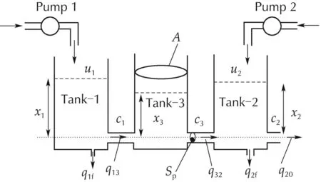
Fig.1 Structure of the three-tank system under consideration.

The discrete-time model will be obtained from the literature[14]by em ploying a simple forward Euler discretization,withTs=0.001:

wherekis the discrete-time instant.

The variables used in this system are given below:

xi(k):Tankiliquid level(m),and 0＜xi(k)＜0.69m,

A:The cross section(m2)of tanks,and all the tanks haveA=0.0154m2.

ci:The outflow coefficients,c1=1,c2=0.8,c3=1.

Sp:The cross section(m2)of the connection pipes,Sp=5×10−5m2.

g:The gravity acceleration(m/s2),g=9.8m/s2.

ui(k):The fluid flow of inlet rate(m3/s)from two pumps,and 0≤ui(k)≤1.2×10−4m3/s,i=1,2.Moreover,whereifif

The phase portrait of the system(56)in normal mode is show n in Fig.2.The state responses of the norm al mode is seen in Fig.3.

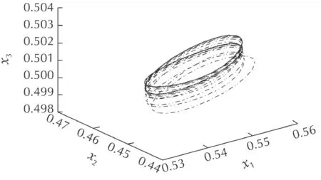
Fig.2 The phase trajectory of the three-tank system in space.

Fig.3 Water levels xi(k).

5.1 Fault modes of three-tanks system

In the three-tank system simulation,the control input term sui(k)are the fluid flow of inlet rate from two pumps.Water levelsxi(k)are in oscillations.The amplitudes of the oscillations are small,which are only about 0.01m.This situation is common in practical application.The purpose of the simulation is to show that accurate NN approximations of the nonlinear system dynamics can be achieved in the local regions near the system equilibrium points.The local NN approximations are then used to detect the faults.

We consider four types of abrupt faults,and also hypothesize every type contains only one fault.The trajectory of fault is close to the normal trajectory when the fault occurs.Moreover,it is assumed that the measurements of the water levelsxi(k),which are influenced by a pump fault or a leakage.The behaviour of the system(56)in the following situations:

1)Normal mode:The system is not faulty.

In this simulation,thexi(k+1)subsystem is considered to be unknown,i.e.,state equations represent the general fault function of normal mode.

2)Fault mode 1:Actuator fault in pum p 1.

We consider a simple multiplicative actuator fault in pump1by lettingwhereu1(k)is the supp ly flow rate in the non-fault case,and α1is the parameter characterizing the magnitude of the fault.For α1=1,we have the non-fault situation in pump1,whereas α1=0 imp lies that the pump is completely faulty,in the sense that there is no flow.For this simulation,α1=0.8.

3)Fault mode 2:Actuator fault in pump 2.

Analogously to the case of a fault in pump 1,we have

4)Fault mode 3:Leakage in tank 1.

5)Fault m ode 4:Leakage in tank 2.

These faults are presented only as representative examples of all the countless faults which can take place in the system.The case of incipient faults is completely analogous and is not addressed here for the sake of brevity.

Consider the same initial condition isx(0)=[x1(0)x2(0)x3(0)]T=[0.54 0.45 0.5]T.The phase portrait and state responses of the fault modes are seen in Figs.4–11.

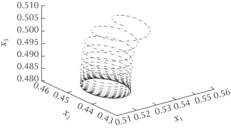
Fig.4 The phase trajectory of the fault mode 1.

Fig.5 Water levels xi(k)of the fault m ode 1.

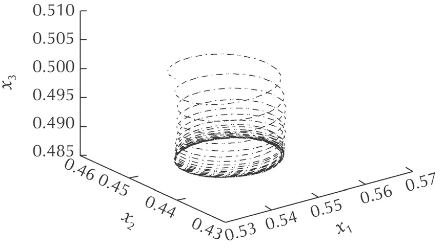
Fig.6 The phase trajectory of the fault mode 2.

Fig.7 Water levels xi(k)of the fault mode 2.

Fig.8 The phase trajectory of the fault mode 3.

Fig.9 Water levels xi(k)of the fault mode 3.

Fig.10 The phase trajectory of the fault mode 4.

Fig.11 Water levels xi(k)of the fault mode 4.

5.2 Training phase

For the discrete-time system(56),the following dynamical RBF networks are em ployed to learn the normal and fault m odes:

The RBF networkwith nodesN=18×11×28 nodes are constructed to learn the unknown system dynamic in the first state equation in normal and fault modes,whereas the RBF networkwith the same nodes are constructed to learn the system dynamic in the second state equation in normal and fault modes,s=0,...,4.The centers of RBF network evenly spaced on[0.510,0.580]×[0.430,0.465]×[0.475,0.505]with the w idths η=0.0025.Figs.3,5,7,9 and 11 show the NN inputsx1(k),x2(k)andx3(k)for training the normal and fault m odes,respectively.

Consider the actuator fault of fault m ode 1,with the initial condition is,fix the system parameter as α1=0.8 to generate a periodic discrete-time sequence.Using the dynamical RBF networks(57)to learn the general fault functions,Fig.12 displays the trajectory of fault mode 1 and NN coverage in space.

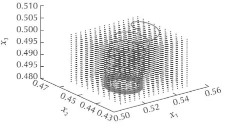
Fig.12 NN coverage of the fault mode 1.

Fig.13 show that convergence of partial NN parameter to their optimal values and locally accurate approximation of system dynamics are implemented in the process of training fault m odes.The learned know ledge is stored in constant RBF networks.

Fig.13 Partial NN parameter convergence of

Simulation results for training of other faults and modes are similar to the above fault mode,and are omitted here due to the limitation of space.

6 Fault detection phase

We consider two types of monitored system with abrupt fault,and also hypothesize every type contains only one fault.

Assume that for the monitored system 1,a fault occurs atk0=250 steps due to the multiplicative actuator fault in pump 1.the parameter of the fault magnitude isThe phase trajectory and states of the monitored system 1 are shown in Figs.14 and 15.

Fig.14 The phase trajectory of the monitored system 1.

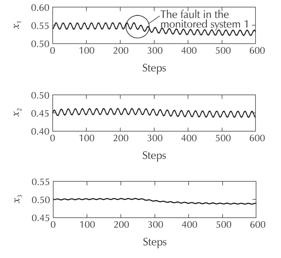
Fig.15 Water levels xi(k)of the monitored system 1.

Assume that for the monitored system 2,a leakage fault occurs atk0=250steps with cross sectionin tank 1.The phase trajectory and states of the monitored system 2 are shown in Figs.16 and 17.The process for learning other actuator and plant faults are similar to those detecting results of the monitored system s 1 and 2,and are omitted here.

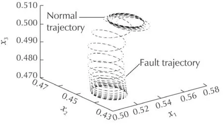
Fig.16 The phase trajectory of the monitored system 2.

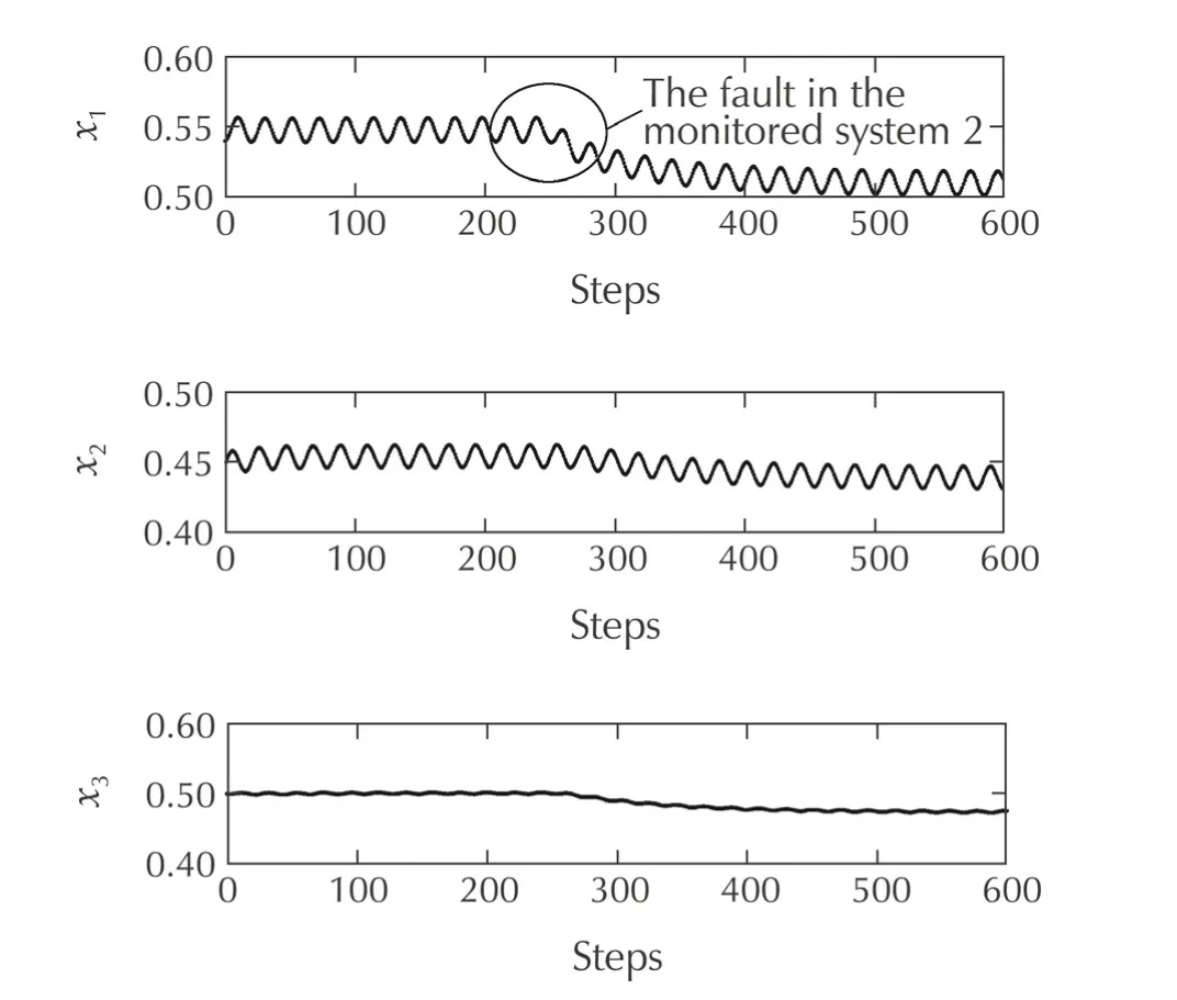
Fig.17 Water levels xi(k)of the monitored system 2.

Consider fault m odes 0,1 and 3 because of the monitored fault occurs at pump 1.Three RBF NN estimators are constructed for detecting the first state equation of the monitored system:

whereas three RBF NN estimators are constructed for detecting the second state equation of the monitored system:

whereare the state of the estimators,x1andx2are the state of the monitored system s.The parameterb1=b2=0.5 is designed.andare the residuals.

According to(20),the averageL1norm of the residuals is calculated withK=30steps.The detection time is yielded because of the choice of the preset period constant of the monitored system(i.e.,K)for calculating the averageL1norm of the residuals.

For the first state equation of the monitored system 1,the averageL1normare shown in Fig.18.becomes smaller thanat approximatelyKd=319steps.It is m ean that the test fault is detected atKd=319steps,and the fault detection tim esteps.

Fig.18 The average L1 normof the monitored system 1.

For the first state equation of the monitored system 2,the averageL1normare shown in Fig.19.becomes smaller thanat approximatelyKd=290steps.Thus the test fault is detected atKd=290 steps,and the fault detection tim ekd=Kd−k0=40 steps.

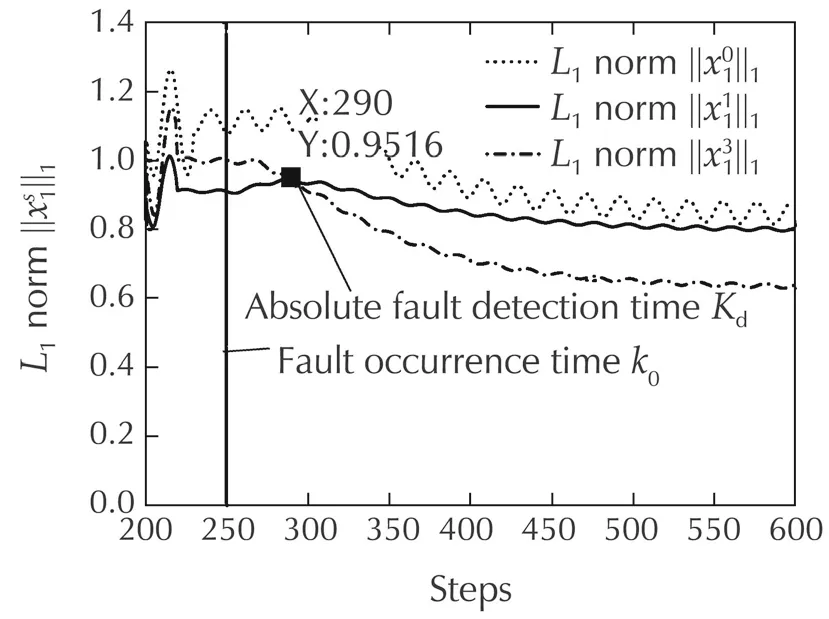
Fig.19 The average L1 normof the monitored system 2.

7 Conclusions

In this paper,an approach has been proposed for fault detection of nonlinear discrete-time system s based on the recently proposed deterministic learning theory.First,the discrete-time dynamical RBF network with an extended weight update law has been em ployed to locally-accurately approximate the general fault function(i.e.,the internal dynamic)via deterministic learning.The obtained know ledge of system dynamics has been embedded to construct a bank of estimators,and a set of residuals have been obtained and used to measure the differences between the dynamics of the monitored system and the dynamics of the trained system s.Second,a fault detection decision scheme has been presented by comparing the magnitude of residuals.Subsequently,the fault detectability analysis has been carried out and the upper bound of detection time has been derived.Finally,a simulation example has been given to illustrate the effectiveness of the proposed scheme.

Future research effort will be devoted to address several issues including:i)performance analysis of the proposed fault detection scheme;ii)fault isolation for nonlinear discrete-time system s;iii)fault detection and isolation for closed-loop discrete-time system s;iv)fault tolerant control design for nonlinear discrete-time system s;and v)detection of simultaneous faults may occur at the same time.

References

[1]J.Chen,R.J.Patton.Robust Model-based Fault Diagnosis for dynamic System s.Boston:Kluwer,1999.

[2]S.Simani,C.Fantuzzi,R.J.Patton.Model-based Fault Diagnosis in dynamic System s Using Identification Techniques.London:Springer,2003.

[3]H.Hamm ouri,M.Kinnaert,E.H.Yaagoubi.Observer-based approach to fault detection and isolation for nonlinear system s.IEEE Transactions on Automatic Control,1999,44(10):1879–1884.

[4]C.Edwards,S.K.Spurgeon,R.J.Patton.Sliding mode observers for fault detection and isolation.Automatica,2000,36(4):541–553.

[5]C.D.Persis,A.Isidori.A geometric approach to nonlinear fault detection and isolation.IEEE Transactions on Automatic Control,2001,46(6):853–865.

[6]B.Jiang,M.Staroswiecki,V.Cocquempot.Fault diagnosis based on adaptive observer for a class of nonlinear system s with unknown parameters.International Journal of Control,2004,77(4):415–426.

[7]F.Caccavale,P.Cilibrizzi,F.Pierri,et al.Actuators fault diagnosis for robot manipulators with uncertain model.Control Engineering Practice,2009,17(1):146–157.

[8]Q.Shen,B.Jiang,V.Cocquempot.Fault tolerant control for T-S fuzzy system s with application to near space hypersonic vehicle with actuator faults.IEEE Transaction on Fuzzy System s,2012,20(4):652–665.

[9]L.Yao,J.Qin,H.Wang,et al.Design of new fault diagnosis and fault tolerant control scheme for non-Gaussian singular stochastic distribution system s.Automatica,2012,48(9):2305–2313.

[10]H.Wang,Z.Huang,S.Daley.On the use of adaptive updating rules for actuator and sensor fault diagnosis.Automatica,1997,33(2):217–225.

[11]M.M.Polycarpou,P.A.Ioannou.Modelling,identification and stable adaptive control of continuous-time nonlinear dynamical system s using neural networks.Proceedings of the American Control Conference,Evanston:American Automatic Control Council,1992:36–40.

[12]M.A.Demetriou,M.M.Polycarpou.Incipient fault diagnosis of dynamical systems using online approximators.IEEE Transactions on Automatic Control,1998,43(11):1612–1617.

[13]M.M.Polycarpou,A.B.Trunov.Learning approach to nonlinear fault diagnosis:detectability analysis.IEEE Transactions on Automatic Control,2000,45(4):806–812.

[14]X.Zhang,M.M.Polycarpou,T.Parisini.A robust detection and isolation scheme for abrupt and incipient faults in nonlinear system s.IEEE Transactions on Automatic Contro l,2002,47(4):576–593.

[15]Z.Mao,B.Jiang,P.Shi.Fault-tolerant control for a class of nonlinear sampled-data system s via a Euler approximate observer.Automatica,2010,46(11):1852–1859.

[16]F.Caccavale,F.Pierri,L.Villani.Adaptive observer for fault diagnosis in nonlinear discrete-time system s.Journal of dynamic System s,Measurement and Control,Transactions of the ASME,2008,130(2):DOI 10.1115/1.2837310.

[17]T.T.Balaje,S.Jagannathan.An online approxim ator-based fault detection framework for nonlinear discrete-time system s.Proceedings of the 46th IEEE Conference on Decision and Control,Piscataway:IEEE,2007:2608–2613.

[18]T.T.Balaje,S.Jagannathan.A model-based fault-detection and prediction scheme for nonlinear multivariable discrete-time system s with asymptotic stability guarantees.IEEE Transactions on Neural Networks,2010,21(3):404–423.

[19]M.G.Riccardo,G.Ferrari,T.Parisini,et al.Distributed fault detection and isolation of large-scale discrete-time nonlinear system s:an adaptive approximation approach.IEEE Transactions on Automatic Control,2012,57(2):275–290.

[20]C.Wang,D.J.Hill.Learning from neural control.IEEE Transactions on Neural Networks,2006,17(1):30–46.

[21]C.Wang,D.J.Hill.deterministic learning and rapid dynamical pattern recognition.IEEE Transactions on Neural Networks,2007,18(3):617–630.

[22]C.Wang,D.J.Hill.deterministic Learning Theory for Identification,Recognition and Control.Boca Raton:CRC Press,2009.

[23]C.Wang,T.Chen.Rapid detection of small oscillation faults via deterministic learning.IEEE Transactions on Neural Networks,2011,22(8):1284–1296.

[24]C.Wang,B.Wen,W.Si,et al.Modeling and detection of rotating stall in axial flow compressors–Part I:Investigation on high-order M-G models via deterministic learning.Acta Automatica Sinica,2014,40(7):1265–1277.

[25]W.Zeng,C.Wang.Gait recognition across different walking speeds via deterministic learning.Neurocomputing,2015,152:139–150.

[26]W.Zeng,C.Wang.Classification of neurodegenerative diseases using gait dynamics via deterministic learning.Inform ation Sciences,2015,317:246–258.

[27]X.Dong,C.Wang,J Hu.Electrocardiogram(ECG)pattern modeling and recognition via deterministic learning.Control Theory and Technology,2014,12(4):333–344.

[28]E.W.Bai,S.S.Sastry.Persistency of excitation,sufficient richness and parameter convergence in discrete time adaptive control.System s&Contro l Letters,1985,6(3):153–163.

[29]T.Liu,C.Wang,D.J.Hill.deterministic learning and rapid dynamical pattern recognition of discrete-time system s.Proceedings of the IEEE International Symposium on Intelligent Control,Piscataway:IEEE,2008:1091–1096.

[30]C.Wang,T.R.Chen,T.Liu.deterministic learning and databased modeling and control.Acta Automatica Sinica(Chinese),2009,35(6):693–706.

[31]C.Yuan,C.Wang.Design and performance analysis of deterministic learning of sampled-data nonlinear system s.Science China Inform ation Sciences,2014,57(18):DOI 10.1007/s11432-012-4731-3.

[32]L.P.Shilnikov,A.L.Shilnikov,D.V.Turaev,et al.Methods of Qualitative Theory in Nonlinear dynamics–Part II.Singapore:World Scientific,2001.

[33]C.Wang,T.Chen,G.Chen,et al.deterministic learning of nonlinear dynamical system s.International Journal of Bifurcation and Chaos,2009,19(4):1307–1328.

[34]V.H.Garnier,A.H.Epstein,E.M.Greitzer.Rotating wave as a stall inception indiccation in axial compressors.ASME Journal of Turbomachinery,1991,113(2):1–9.

[35]J.H.Deane,D.C.Ham ill.Instability,subharmonics,and chaos in power electronic system s.IEEE Transactionson Power Electronics,1990,5(3):260–268.

[36]S.R.Samantaray,P.K.Dash,S.K.Upadhyay.Adaptive Kalmanfiter and neural network based high impedance fault detection in power distribution networks.Electrical Power and Energy Systems,2009,31(3):167–172.

[37]A.R.Messina.Inter-area Oscillations in Power Systems.New York:Springer,2009.

[38]H.Yin,P.Wang,T.Alpcan,et al.Hopf bifurcation and oscillations in a communication network with heterogeneous delays.Automatica,2009,45(10):2358–2367.

[39]H.G.Hosseini,D.Luo,K.J.Reynolds.The comparison of different feed forward neuralnet work architectures for ECG signal diagnosis.Medical Engineering&Physics,2006,28(4):372–378.

[40]C.Yuan,C.Wang.Pesistency of excitation and performance of deterministic learning.System s&Control Letters,2011,60(12):952–959.

[41]U.Altinisik,M.Yildirim.A new fault tolerant control approach for the three-tank system using data m ining.Computers&Electrical Engineering,2012,38(6):1627–1635.