Symmetric Coupling of the Meshless Galerkin Boundary Node and Finite Element Methods for Elasticity
2014-04-17XiaolinLi
Xiaolin Li
1 Introduction
Meshless(or meshfree)methods have been proposed and achieved remarkable progress in the past two decades[Atluri(2004);Li and Liu(2004);Liu(2009)].Compared with traditional mesh-based numerical methods such as the finite element method(FEM)and the boundary element method(BEM),meshless methods get rid of,or at least alleviate,the difficulty of meshing and remeshing the entire structure by simply adding or deleting nodes.Meshless methods have developed so fast that they are applied successfully to a variety of science and engineering problems.
The moving leastsquare(MLS)is an approximation scheme of constructing continuous functions from a set of unorganized sampled point values.Since the numerical approximations start from scattered nodes instead of elements,the MLS scheme is one of the most extensively used schemes to form the meshless shape functions.Some MLS-based meshless methods,such as the element-free Galerkin(EFG)method[Liu(2009)],theh-pmeshless method[Duarte and Oden(1996)],the moving least square reproducing kernel method(MLSRKM)[Li and Liu(1996)]and the meshless local Petrov-Galerkin(MLPG)method[Sladek,Stanak,and Han(2013)]have been developed.They are domain type,as the FEM,in which the problem domain is discretized by nodes.
The boundary integral equation(BIE)is an important and attractive computational tool as it can reduce the dimensionality of the considered problem by one.The boundary type meshless methods are developed by the combination of the meshless idea with BIEs,such as the boundary node method(BNM)[Mukherjee and Mukherjee(2005)],the boundary cloud method(BCM)[Li and Aluru(2002)],the hybrid boundary node method(HBNM)[Miao,He,and Luo(2012)]and the boundary face method(BFM)[Zhang,Qin,Han,and Li(2009)].In these methods,the MLS scheme is used to generate the shape functions on the boundary of a domain.These methods take the advantages of both the BIE in dimension reduction and the MLS scheme in elements elimination.However,since the MLS scheme lacks the delta function property,they cannot exactly satisfy boundary conditions.The technique used in the BNM to impose boundary conditions doubles the number of system equations.This technique is also used in the BCM,the HBNM and the BFM,together with the addition of a penalty formulation.
Liew,Cheng,and Kitipornchai(2006)developed an improved MLS scheme that uses weighted orthogonal polynomials as basis functions.The improved MLS scheme has been introduced into BIEsto develop a boundary element-free method(BEFM).Because the improved MLS scheme still lacks the delta function property,boundary conditions in the BEFM are implemented with constraints.To construct meshless shape functions with delta function properties,Li and Li(2014)discussed mathematically an improved interpolating MLS scheme and developed an interpolating BEFM for potential problems and unilateral problems.Besides,Liuet al.developed the point interpolation method(PIM)and introduced it into BIEs to produce boundary PIMs[Gu and Liu(2003);Liu(2009)].Recently,Li(2014)developed a dual boundary node method(DBNM)for implementation of boundary conditions in BIEs-based meshless methods.In the DBNM,boundary conditions are introduced directly into dual BIEs including the conventional BIE and hypersingular BIE.Consequently,the DBNM can apply boundary conditions directly and easily,and the number of both unknowns and system equations in the DBNM is only half of that in the BNM.
Li and Zhu(2009b)and Li(2011a)developed a boundary type meshless method called the Galerkin boundary node method(GBNM).It combines the MLS scheme with a variational(weak)version of BIEs.The MLS scheme is implemented for constructing the trial and test functions of the variational form,thus only the boundary of a problem domain is discretized by a set of scattered nodes instead of elements.Unlike other MLS-based methods mentioned above,boundary conditions in the GBNM do not present any difficulty and can be implemented with ease via multiplying the MLS shape function and integrating on the boundary.The GBNM has been applied to elastic problems with pure displacement boundary conditions[Li and Zhu(2009a)]and pure traction boundary conditions[Li and Li(2013)].It is well known that mixed boundary value problems play an important role in many different applications of physics,mechanics and engineering.In this paper,the GBNM is further developed for solving elastic problems with mixed boundary conditions of displacement and traction type.
In contrast with other boundary type meshless methods aforementioned,another outstanding feature of the GBNM is the conservation of the symmetry and positive definiteness of the variational problems in the process of numerical implementation.The property of symmetry can be an added advantage in coupling the GBNM with other numerical methods.Some coupled methods,such as the coupled BEM and FEM[Brebbia and Georgion(1979);Stephan(2004);Beer(2001);Ganguly,Layton,and Balakrishna(2000);Haas and Kuhn(2003);Dong and Atluri(2012a,b,2013)],the coupled EFG and FEM[Belytschko and Organ(1995)],the coupled MLPG and FEM[Liu(2009)],the coupled MLPG and BEM[Tadeu,S-tanak,and Sladek(2013)],the coupled improved EFG and BEM[Zhang,Liew,and Cheng(2008)],and the coupled reproducing kernel particle boundary element-free method(RKPBEFM)and FEM[Qin and Cheng(2008)],have been developed.In this paper,based on the coupled techniques propose by Ganguly,Layton,and Balakrishna(2000),Haas and Kuhn(2003),Zhang,Liew,and Cheng(2008)and Qin and Cheng(2008),a direct symmetric coupling of the GBNM and the FEM is also developed for elasticity problems.In the present coupled method,the resulting coupling matrix is symmetric and positive definite.
Error analysis and convergence study,which ensure convergence of numerical methods,are crucial in meshless research.The associated mathematical proofs guarantee that meshless methods will converge to the true solution.Over the past two decades,it has been developed so fast in the areas of meshless research from both computational and mathematical point of views.A large amount of research has been devoted to deriving error estimation for MLS-based domain type meshless methods such as theh-pmeshless method[Duarte and Oden(1996)],the MLSRKM[Li and Liu(1996)]and the finite point method[Cheng and Cheng(2008)].Nevertheless,although boundary type meshless methods perform very well in practice,not much is rigorously known on the mathematical foundation of these schemes.Until now,a rigorous mathematical analysis of boundary type meshless methods was given for the GBNM for potential problems[Li and Zhu(2009b);Li(2011a,2012)],for Stokes problems[Li and Zhu(2009c);Li(2011b)]and for elasticity problems with pure displacement or traction boundary conditions[Li and Zhu(2009a);Li and Li(2013)].Thus,one aim of this paper is to provide a solid mathematical foundation to the GBNM for the mixed boundary value problems of elastostatics.Besides,the error analysis and convergence study of the coupled GBNM-FEM are also presented in Sobolev spaces.
An outline of this paper is as follows.In Section 2 we give a detailed numerical implementation and error analysis of the GBNM for elasticity problems with mixed boundary conditions.Section 3 deals with the GBNM-FEM coupling approach and the corresponding error analysis.Numerical examples are presented in Section 4.Section 5 contains conclusions.
2 The GBNM for mixed elasticity problems
2.1 BIEs
Let Ω be a bounded or unbounded domain in Rd(d=2,3)with boundary Γ =Γu∪Γt,Γu∩Γt=/0,Γu/=/0,with given displacement data on Γu,and traction data on Γt.In linear elasticity for isotropic materials,the governing equation is

where u=(u1,u2,···,ud)Tis the displacement field;λandµare classical Lamé constants;∆,∇ and∇·stand for the Laplacian,gradient and divergence operators,respectively.Suitable boundary conditions are associated with this field equation.They can be of the following types:


Eqs.(1)-(3)compose the standard mixed boundary value problem of linear elasticity.The associated BIE is[Zhu and Yuan(2009)]


Here,I is the identity matrix,r=|x-y|,E(x,y)=-lnrford=2 andE(x,y)=1?rford=3.LetTbe the differential operator which transforms a displacement field in Ω into the corresponding traction on its boundary.When the derivatives are taken with respect to x or y,then we denote it byTxandTy,respectively.Under this notation,Ty(x,y)=(TyU(x,y))Tis the strongly singular fundamental solution.
In Eq.(4),letting x tend to Γ,we obtain the strongly singular displacement BIE

Then applying the operatorTxto Eq.(5)yields the hypersingular traction BIE

In Eqs.(5)and(6),we have used the standard notations for the boundary integral operators defined on Γ,
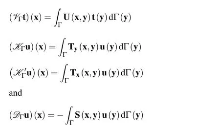
Here,Tx(x,y)=TxU(x,y)and S(x,y)=TxTy(x,y)are the strongly singular and hypersingular fundamental solutions,respectively.
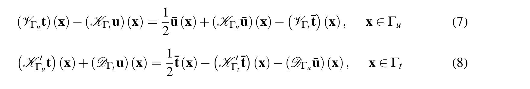
Obviously,the kernel functions are symmetric,i.e.,U=UT,S=STand Ty=TTx.Thus,to find the complete Cauchy data[u,t]|Γand to achieve a symmetric formulation,Eq.(5)is used where the boundary traction t is unknown,while Eq.(6)is used where the boundary displacement u is unknown.Then according to boundary conditions(2)and(3),we get the following BIEs:
2.2 Variational formulation
Let

denote the usual Sobolev space of functions defined on Γ[Zhu and Yuan(2009)].In the following,we often write‖·‖τ,Γfor the Sobolev norm‖·‖Hτ(Γ).
Besides,let H-τ(Γ)be the dual space of Hτ(Γ)with respect to the duality〈·,·〉Γwhich is defined for functionswandvby

Then Eqs.(7)and(8)lead to the following variational problem:
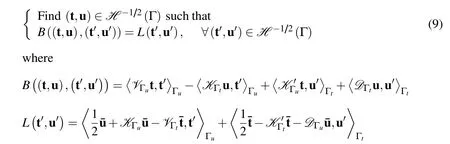
The unique solvability of the variational problem(9)follows from the continuity of the boundary integral operators introduced above and the coerciveness of the operatorsVandD.
2.3 Approximation
Let{xi}Ni=1be a set ofNboundary nodes xi∈Γ and let


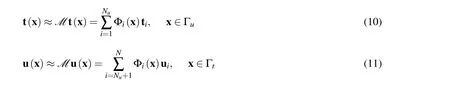
whereMis an approximation operator,tiand uiare the nodal values,and Φiis the shape function of the MLS approximation,which can be defined as[Li and Zhu(2009b);Li(2011a)]
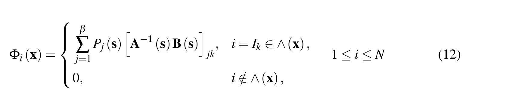
where s is a local coordinate of the boundary point x on Γ,Pj(s)is a basis of orderβconsisting of monomials in s,∧(x)={I1,I2,···,Iκ}is the set of the global sequence numbers of boundary nodes that lie on the influence domain of x,and the matrices A(s)and B(s)are defined by

In what follows,we assume that there exists a positive numberγ≥1?2 such that the chosen weight functionwiisγ-times continuously differentiable and the boundary Γ isγ-times piecewise continuous.Then we can conclude that the MLS shape function Φiisγ-times continuously differentiable[Liand Zhu(2009b);Li(2011a)].

be the meshless space.Then the approximation of the variational problem(9)is

2.4 Discretization
Inserting Eqs.(10)and(11)into the variational problem(14),we get the following linear algebraic equations


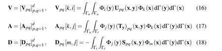
for allk,i=1,2,···,Nuandm,j=Nu+1,Nu+2,···,N.The components of the right-hand side are given by

for allk=1,2,···,Nuandm=Nu+1,Nu+2,···,N.
From the symmetry of the kernel functions and the coerciveness of the operatorsVandD,we conclude that the block matrices V and D are symmetric and positive definite.Hence,the stiffness matrix in Eq.(15)is block skew-symmetric and positive definite.Then,one can solve Eq.(15)by a generalized Krylov subspace method such as the generalized minimum residual method(GMRES).Since this method can not utilize symmetry and positive definiteness simultaneously and sufficiently,equivalent system equations deserve to be established for the practical numerical implementation.
On the other hand,the symmetry and positive definiteness of the block matrix V indicate that it is invertible.Thus,Xtcan be obtained from the first of Eq.(15)as

Then,inserting Eq.(21)into the second of Eq.(15)leads to the Schur complement system

The stiffness matrix in Eq.(22)is symmetric and positive definite,a property that enables the use of more efficient equation solvers and therefore leads to substantial reductions in solution time.Moreover,this property can be an added advantage in coupling the GBNM with the FEM.After solving the reduced system(22),the unknown vector Xtcan be computed in a post processing step via Eq.(21)from the now known vector Xu.Finally,the yet unknowns t on Γuand u on Γtcan be computed using Eqs.(10)and(11),respectively.Then,the approximate solution uhof the mixed elastic problem(1)-(3)can be computed from Eq.(4)as

Eqs.(16)-(20)and(23)have integrations over the boundary.As in many other meshless methods such as the EFG and the BNM,cells are used in this research to approximate the boundary and carry out numerical integration.It is worth mentioning that cells are used just for integration,and pose no restriction on shape or compatibility.In these integrations,if x and y belong to distinct cells,the integrands are regular and thus,the associated double integrals can be evaluated by usual Gaussian quadrature formulas.Otherwise,these double integrals are weakly singular,strongly singular or hypersingular.There have been various regularization procedures proposed in the past to handle various singular integrals.Li(2012)developed a technique to tackle the weakly singular,strongly singular and hypersingular integrations simultaneously.This technique is attractive and is used to carry out the singular integrations in this research.
2.5 Error analysis
In this subsection,we will estimate the error of using the GBNM for solving the mixed elastic problem(1)-(3).In what follows,byCwe will denote a general constant which is independent ofhand may have different values at different occurrences.
Lemma 2.1(Li and Zhu(2009b);Li(2011a))Let M be the MLS approximation operator and let P be the L2-projection onto H h,then for anyv∈Hm+1(Γ)with0≤m≤γ,we have

Theorem 2.1Let(t,u)and(th,uh)be the solutions of variational problems(9)and(14),respectively.Then if(t,u)∈H m(Γ),we have
Proof.Subtraction Eq.(14)from Eq.(9)leads to

then using(Pt,Mu)-(th,uh)∈H hyields

According to the coerciveness and continuity of the bilinear formB(·,·),we have

Gathering Eqs.(25)-(27)and using Lemma 2.1 we finally obtain

which completes the proof.
Theorem 2.2Under the conditions of Theorem 2.1,

Proof.From the duality argument it follows that

SinceP(τ,µ)∈H h,from Eq.(24)one gets
B((t,u)-(th,uh),(τ,µ))=B((t,u)-(th,uh),(τ,µ)-P(τ,µ))
Then using the continuity ofB(·,·),Theorem 2.1 and Lemma 2.1 yields

Finally,inserting Eq.(29)into Eq.(28)ends the proof.
Theorem 2.3Letuanduh be defined by Eqs.(4)and(23),respectively.Assume that(t,u)∈H m(Γ)with1?2≤m≤γ.Then for anyx∈Ωwith ℓx=miny∈Γ|x-y|≥δ>0,we have

Proof.Subtraction Eq.(23)from Eq.(4)yields
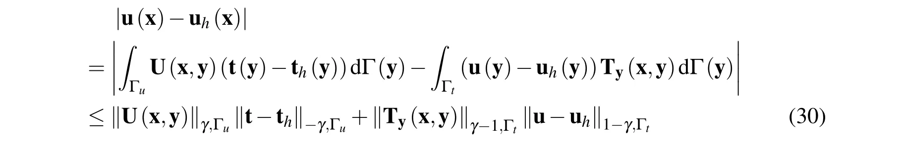
Usingℓx≥δ>0,we have

Thus,substituting Eq.(31)into Eq.(30)and invoking Theorem 2.2 end the proof.Theorem 2.3 indicates that the approximate solution obtained by the meshless GBNM converges to the analytical solution of the elastic problem(1)-(3).The same type of estimate can be obtained for the stress tensorσ.More specifically,we have
Theorem 2.4Let σ be the exact stress solution of the elastic problem(1)-(3)and let σh be the corresponding GBNM solution,then under conditions of Theorem 2.3,

Theorems 2.3 and 2.4 indicate that the errors of stress and displacement in the meshless GBNM are all of the same convergence rate.
Furthermore,the convergence can be established in energy norms.
Theorem 2.5Letuanduh be defined by Eqs.(4)and(23),respectively.If(t,u)∈H m(Γ)with1?2≤m≤γ,then

Proof.Since Eq.(4)defines an isomorphism fromH-1/2(Γ)ontoH1(Ω),we have

The proof is completed via invoking Theorem 2.1.
3 Coupling of the GBNM and the FEM
3.1 Coupled formulation
As shown in Fig.1,a bounded or unbounded problem domain Ω is decomposed into two disjoint sub-domains,ΩGand ΩF,with the GBNM-FEM coupling interface ΓI.The GBNM is used in ΩGand the FEM is used in ΩF.Without loss of generality,it is assumed that both displacement and traction boundary conditions are given on ΓGand ΓF.The boundaries of ΩGand ΩFare denoted as ΓG= ΓuG∪ΓtG∪ΓIand ΓF= ΓuF∪ΓtF∪ΓI,respectively.Note that if the problem domain Ω is unbounded,as shown in Fig.1(b),both the displacement boundary Γuand traction boundary Γtare empty.We consider the model boundary value problems as


Figure 1:The coupling domain of the GBNM and the FEM.(a)the problem domain Ω is bounded and(b)the problem domain Ω is unbounded.


Then,as in Sections 2.2 and 2.4,evaluating Eqs.(36)and(37)in the sense of Galerkin yields
where TIand Tuare the traction vector at the nodes on ΓIand ΓuG,respectively;UIand Utare the displacement vector at the nodes on ΓIand ΓtG,respectively.In the matrices Vij,Aijand Dij,the first index denotes the position of the source point x and the second index stands for the position of the field point y.
Since both the displacements and tractions are unknown on the interface ΓI,applying Eqs.(5)and(6)for x∈ΓIwe gain
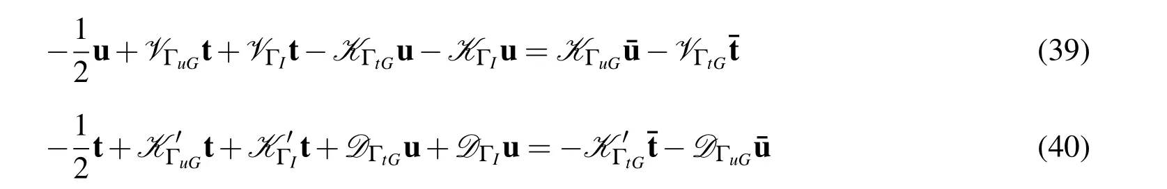
Then evaluating Eqs.(39)and(40)in the sense of Galerkin yields

According to the scheme used for evaluating an equivalent nodal force[Beer(2001)],we can define a vector of equivalent nodal forces on the interface ΓIas

As in Section 2.4,Eq.(42)can be transformed to the following Schur complement system by eliminating the traction vectors,
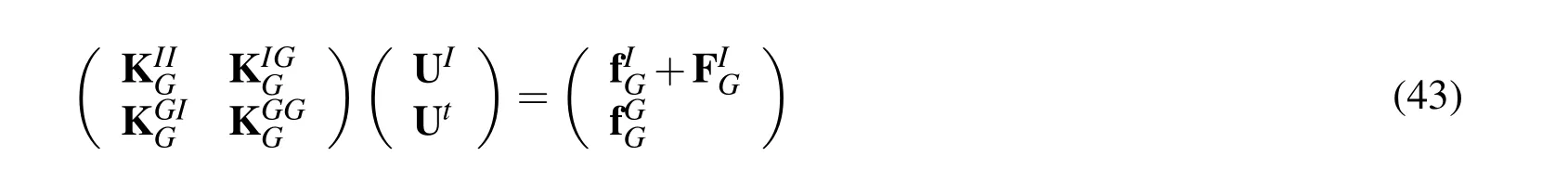
Eq.(43)correlates the nodal displacements with nodal forces.
On the other hand,the FEM sub-domain ΩFyields the following system of equation by the well-known finite element implementation,

where KFis the domain stiffness matrix,U and FFare the nodal displacements and nodal forces,respectively.This equation can be split into two parts corresponding to a region containing the interfacial degrees of freedom and a region containing the non-interfacial degrees of freedom,

Moreover,the compatibility and equilibrium conditions on the coupling interface ΓImust be satisfied.Therefore,the displacements on ΓIfor ΩFand ΩGshould be equal,i.e.


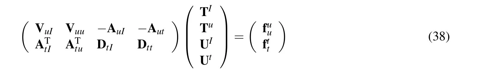
Finally,combining Eqs.(43)and(44),in view of Eqs.(45)and(46),we obtain the coupled equations as follows:
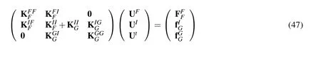
Since the FEM matrix in Eq.(44)is obtained from the usual energy based FEM approaches,the resultant matrix is symmetric and positive definite.The sum of the symmetric and positive definite matrices continues to be symmetric and positive definite.Thus the resulting coupling matrix presented in Eq.(47)is symmetric and positive definite.
3.2 Error analysis
In this subsection,we will estimate the error of using the symmetric coupled GBNMFEM for solving the mixed elastic problem(32)-(35).In what follows,letube the exact displacement solution of the elastic problem and letuhbe the approximated displacement obtained by the GBNM,the FEM or the coupled GBNM-FEM.
In the GBNM sub-domain ΩG,using Theorem 2.5 we have
Theorem 3.1Let hG be the spacing of boundary nodes in the GBNM sub-domainΩG.Then

In the FEM sub-domain ΩF,let us use a regular partition of the interior domain ΩFand lethFdenote the maximum of the longest element sides.On these elements,letHFdenote a finite dimensional subspaces ofH1(ΩF),satisfying

Theorem 3.2The error estimation in the FEM sub-domainΩF is

As stated in the previous section,when the coupled GBNM-FEM is used,the problem domain Ω is decomposed into two disjoint sub-domains,ΩGand ΩF.Thus,

As a consequence,the error estimation of the coupled GBNM-FEM can be established by combining Theorems 3.1 and 3.2.
Theorem 3.3The error estimation in the problem domainΩis

4 Numerical examples
4.1 Examples of the GBNM
Two examples are selected to demonstrate the applicability of the GBNM for elasticity problems.
The first example that is considered is a three-dimensional problem in a cubic domain.The cube is bounded by the planesx1=±1,x2=±1 andx3=±1.The following analytical solution is used,

Displacements are imposed on facesx3=±1 and boundary tractions on all other faces.The material constants that are used in our analysis are Young’s modulusE=1.0 and Poisson’s rationν=0.25.
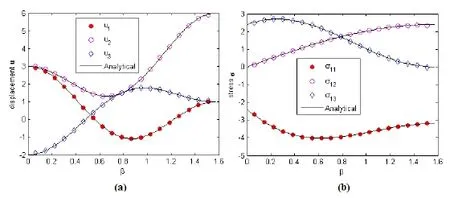
Figure 2:Results of(a)displacement u and(b)stress σ for the cubic problem.
Fig.2 shows a comparison between the numerical results with the analytical solutions for displacement u and stressσalong the arc given by the formulasx1=sinβ,x2=0,x3=cos(2β),β∈[0,0.5π].In this analysis,the cubic surface is discretized using 48 distributed nodes.It is clearly shown that the numerical results agree very well with the analytical ones.
To investigate the convergence of the present method,three different nodal arrangements of 48,192 and 768 boundary nodes have been used.Fig.3 shows the log-log plot of errors with respect to the nodal spacing.As we expected,the numerical results from the proposed meshless method gradually converge to the analytical values along with the decrease of the nodal spacing.

Figure 3:Convergence of the GBNM.

Figure 4:A cylindrical tube subjected to uniform internal pressure.
The second example to be considered is a cylindrical tube subjected to uniform internal pressure.Due to symmetry,only the upper right quadrant of the structure is modeled as shown in Fig.4.The plane stress case is considered,and the parameters are chosen as Young’s modulusE=10,Poisson’s rationν=0.25 and internal pressurep=1.0.Besides,the geometry is chosen asa=1 andb=2.In the polar coordinate system(r,θ),the analytical displacements are[Timoshenko and Goodier(1970)]

and the corresponding stresses are
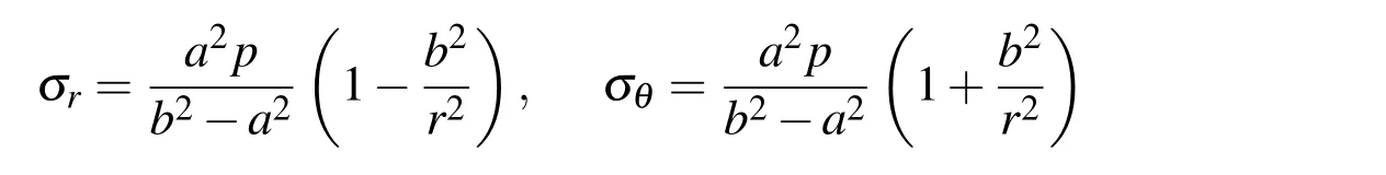
The numerical results by the GBNM are plotted in Fig.5.We again verify these results with the available analytical solution.In this analysis,the boundary is discretized by 60 boundary nodes(12 nodes on AB,CD and AD,and 24 nodes on BC).As expected,these numerical results agree well with the analytical values.

Figure 5:Results of(a)radial displacement ur and(b)stress σ along the radius.
4.2 Examples of the coupled GBNM-FEM
In this subsection,we will present two numerical examples to show the accuracy and efficiency of the coupled GBNM-FEM of this paper.
Consider a beam subjected to a parabolic traction at the free end as shown in Fig.6.The beam is of lengthLand heightH,and has a unit thickness.The beam is assumed to be in a state of plane stress.The analytical solution for this problem is[Timoshenko and Goodier(1970)]


Figure 6:A beam and its computational model.

The beam is separated into two parts.The GBNM is used in the right part and the FEM is used in the left part.The parameters are taken asE=3.0×10⁷kPa,ν=0.3,L=48m,H=12m andP=1000kN in the computation.
The numerical results,which are furnished by the coupled method,are shown in Fig.7 together with the analytical solutions.In this analysis,48 boundary nodes are used in the GBNM region,and 128 quadrangular FEM elements are used in the FEM region.From this figure,we can find that the numerical solutions are in excellent agreement with the analytical solutions.

Figure 7:Results of displacement u2 at x2=0.
The convergence is presented in Fig.8,wherehis equivalent to the maximmum element size in the FEM in this case.We can find that the greater precision of the solution will be obtained when more nodes are selected.

Figure 8:Convergence of the coupled GBNM-FEM.
Next,we consider a semi-infinite soil-structure interaction problem.As shown in Fig.9(a),the FEM is used in the structure region ΩF,and the GBNM is used in the infinite soil foundation region ΩG.As in[Brebbia and Georgion(1979);Qin and Cheng(2008)],the infinite foundation can be treated by truncating the semi-infinite plane at a finite distance from the structure.The computational model is plotted in Fig.9:36 boundary nodes are used in the GBNM region,and 48 triangular elements are used in the FEM region.
Consider five concentrated vertical loads on the top of the structure.Table 1 gives the vertical displacement on the top of the structure.The results obtained using the FEM[Brebbia and Georgion(1979)],the coupled BEM-FEM[Brebbia and Georgion(1979)]and the coupled RKPBEFM-FEM[Qin and Cheng(2008)]are also given in the table for comparison.Although no analytical solutions exist for such a complex problem,the solutions of the presented coupled method are in good agreement with the results of other methods.
5 Conclusions
The meshless GBNM is developed in this paper for the numerical solution of mixed elasticity problems in two and three dimensions.In this method,an equivalent variational form of BIEs is used,thus boundary conditions are applied directly and easily.Another prominent feature of the present approach is that the resulting system matrix is not only symmetric but also positive definite.This paper also examines an efficient symmetric coupling of the GBNM with the FEM.In the coupled method,the resulting coupling matrix is symmetric and positive definite.Theoretical error estimates of the GBNM and the coupled GBNM-FEM are established.From the error analysis,it is shown that the error bound of the numerical solution is directly related to the nodal spacing.Some numerical examples have been given and the numerical results are accurate and are in agreement with the theoretical analysis.

Figure 9:Schematic diagram for the problem of a structure standing on a semiinfinite foundation.(a)The coupled GBNM/FEM model.(b)Meshes and loads on the FEM region.

Table 1:Vertical displacement(×10-4)along top of the structure
Acknowledgement:This work was supported by the National Natural Science Foundation of China(No.11101454),the Educational Commission Foundation of Chongqing of China(No.KJ130626),the Natural Science Foundation Project of CQ CSTC(No.cstc2013jcyjA30001),and the Program of Chongqing Innovation Team Project in University(No.KJTD201308).
Atluri,S.N.(2004):The Meshless Method(MLPG)for Domain&BIE Discretizations.Tech.Science Press,California.
Beer,G.(2001):Programming the Boundary Element Method.Wiley,Chichester.Belytschko,T.;Organ,D.(1995):Coupled finite element-element-free Galerkin method.Computational Mechanics,vol.17,pp.186–195.
Brebbia,C.A.;Georgion,P.(1979): Combination of boundary and finite elements in elastostatics.Applied Numerical Mathematics,vol.3,pp.212–219.
Cheng,R.;Cheng,Y.(2008):Error estimates for the finite point method.Applied Numerical Mathematics,vol.58,pp.884–898.
Dong,L.;Atluri,S.N.(2012): Development of 3D Trefftz voronoi cells with ellipsoidal voids/or elastic/rigid inclusions for micromechanical modeling of heterogeneous materials.CMC:Computer Materials&Continua,vol.30,pp.39–82.
Dong,L.;Atluri,S.N.(2012):SGBEM(using non-hyper-singular traction BIE),and super elements,for non-collinear fatigue-growth analyses of cracks in stiffened panels with composite-patch repairs.CMES:Computer Modeling in Engineering&Sciences,vol.89,pp.417–458.
Dong,L.;Atluri,S.N.(2013):SGBEM Voronoi Cells(SVCs),with embedded arbitrary-shaped inclusions,voids,and/or cracks,for micromechanical modeling of heterogeneous materials.CMC:Computer Materials&Continua,vol.33,pp.111–154.
Duarte,C.A.;Oden,J.T.(1996):H-p clouds—an h-p meshless method.Numerical Methods for Partial Differential Equations,vol.12,pp.675–705.
Ganguly,S.;Layton,J.B.;Balakrishna,C.(2000): Symmetric coupling of multi-zone curved Galerkin boundary elements with finite elements in elasticity.International Journal for Numerical Methods in Engineering,vol.48,pp.633–654.
Gu,Y.T.;Liu,G.R.(2003):Hybrid boundary point interpolation methods and their coupling with the element free Galerkin method.Engineering Analysis with Boundary Elements,vol.27,pp.905–917.
Haas,M.;Kuhn,G.(2003): Mixed-dimensional,symmetric coupling of FEM and BEM,Engineering Analysis with Boundary Elements.Engineering Analysis with Boundary Elements,vol.27,pp.575–582.
Li,F.;Li,X.L.(2014): The interpolating boundary element-free method for unilateral problems arising in variational inequalities.Mathematical Problems in Engineering,vol.2014,pp.Article ID 518727.
Li,G.;Aluru,N.R.(2002): Boundary cloud method:a combined scattered point/boundary integral approach for boundary-only analysis.Computer Methods in Applied Mechanics and Engineering,vol.191,pp.2337–2370.
Li,S.F.;Liu,W.K.(1996):Moving least square reproducing kernel method(II)Fourier analysis.Computer Methods in Applied Mechanics and Engineering,vol.139,pp.159–193.
Li,S.F.;Liu,W.K.(2004):Meshfree Particle Methods.Springer,Berlin.
Li,X.L.(2011): Meshless Galerkin algorithms for boundary integral equations with moving least square approximations.Applied Numerical Mathematics,vol.61,pp.1237–1256.
Li,X.L.(2011):The meshless Galerkin boundary node method for Stokes problems in three dimensions.International Journal for Numerical Methods in Engineering,vol.88,pp.442–472.
Li,X.L.(2012): Application of the meshless Galerkin boundary node method to potential problems with mixed boundary conditions.Engineering Analysis with Boundary Elements,vol.36,pp.1799–1810.
Li,X.L.(2014):Implementation of boundary conditions in BIEs-based meshless methods:A dual boundary node method.Engineering Analysis with Boundary Elements,vol.41,pp.139–151.
Li,X.L.;Li,S.L.(2013):A meshless Galerkin method with moving least square approximations for infinite elastic solids.Chinese Physics B,vol.22,pp.080204.
Li,X.L.;Zhu,J.L.(2009): A Galerkin boundary node method for twodimensional linear elasticity.CMES:Computer Modeling in Engineering&Sciences,vol.45,pp.1–29.
Li,X.L.;Zhu,J.L.(2009):A Galerkin boundary node method and its convergence analysis.Journal of Computational and Applied Mathematics,vol.230,pp.314–328.
Li,X.L.;Zhu,J.L.(2009): A meshless Galerkin method for Stokes problems using boundary integral equations.Computer Method in Applied Mechanics Engineering,vol.198,pp.2874–2885.
Liew,K.M.;Cheng,Y.;Kitipornchai,S.(2006):Boundary element-free method(BEFM)and its application to two-dimensional elasticity problems.International Journal for Numerical Methods in Engineering,vol.65,pp.1310–1332.
Liu,G.R.(2009):Mesh Free Methods:Moving Beyond the Finite Element Method.CRC Press,Boca Raton.
Miao,Y.;He,T.G.;Luo,H.(2012): Dual hybrid boundary node method for solving transient dynamic fracture problems.CMES:Computer Modeling in Engineering&Sciences,vol.85,pp.481–498.
Mukherjee,S.;Mukherjee,Y.(2005):Boundary Methods:Elements,Contours,and Nodes.CRC Press,Boca Raton.
Qin,Y.;Cheng,Y.(2008):Combination of the reproducing kernel particle boundary element-free method and the finite element method for elasticity.Chinese Journal of Solid Mechanics,vol.29,pp.205–211.
Sladek,J.;Stanak,P.;Han,Z.D.(2013):Applications of the MLPG method in engineering&sciences:A review.CMES:Computer Modeling in Engineering&Sciences,vol.92,pp.423–475.
Stephan,E.P.(2004):Coupling of Boundary Element Methods and Finite Element Methods.Encyclopedia of Computational Mechanics,Edited by E.Stein,R.Borst and T.J.R.Hughes,Volume 1:Fundamentals,pp.375–412.
Tadeu,A.;Stanak,P.;Sladek,J.(2013):A coupled BEM-MLPG technique for the thermal analysis of non-homogeneous media.CMES:Computer Modeling in Engineering&Sciences,vol.93,pp.489–516.
Timoshenko,S.P.;Goodier,J.N.(1970):Theory of Elasticity.McGraw-Hill,New York.
Zhang,J.;Qin,X.;Han,X.;Li,G.(2009):A boundary face method for potential problems in three dimensions.International Journal for Numerical Methods in Engineering,vol.80,pp.320–337.
Zhang,Z.;Liew,K.M.;Cheng,Y.(2008):Coupling of the improved elementfree Galerkin and boundary element methods for two-dimensional elasticity problems.Engineering Analysis with Boundary Elements,vol.32,pp.100–107.
Zhu,J.L.;Yuan,Z.Q.(2009):Boundary Element Analysis.Science Press,Beijing.