Voxel-based Analysis of Electrostatic Fields in Virtual-human Model Duke using Indirect Boundary Element Method with Fast Multipole Method

S.Hamada

1　Introduction

Numerical electromagnetic field analyses based on voxel models are widely conducted with the use of the finite difference method,the finite element method,etc.[Dawson,Caputa,and Stuchly(1997);Dawson,Caputa,and Stuchly(1998);Hatada,Sekino,and Ueno(2005)].The merits of the voxel-based analysis include the facile production of realistic models from three-dimensional image data,and the simplicity in data structure suitable for easy storage,handling,and visualiza-tion.Such merits facilitate the analysis of relatively large-scale realistic models,a typical example of which is the human anatomical model made from magnetic resonance images.The voxel-based analysis also has some demerits,a major demerit being the numerical field error due to the staircase approximation of boundaries.Despite such errors,the usefulness of voxel-based analyses,for example the finite difference time-domain(FDTD)analysis,is widely accepted.

Voxel-based analyses with boundary element methods(BEM),which analyze relatively small-scale problems,have often been reported in the past.On the other hand,a voxel-based indirect BEM(IBEM)for relatively large-scale problems that adopts the Laplace kernel fast multipole method(FMM)has been reported by Hamada and Kobayashi(2006)and Hamada(2011,2013).This IBEM analyzed the electrostatic fields in anatomical cubic-voxel models,which describe the conductivities of biological tissues,with the accuracy comparable to those by the finite difference method and the quasi-static FDTD method[Hirata,Yamazaki,Hamada,Kamimura,Tarao,Wake,Suzuki,Hayashi,and Fujiwara(2010)].In general,the IBEM can be applied to static field problems.

The resolution of anatomical voxel models used in computational dosimetry is increasingly getting finer.For example,the foundation for research on information technologies in society(IT’IS Foundation)provides an adult male model called Duke[Christ,Kainz,Hahn,Honegger,Zefferer,Neufeld,Rascher,Janka,Bautz,Chen,Kiefer,Schmitt,Hollenbach,Shen,Oberle,Szczerba,Kam,Guag,and Kuster(2010)].It is originally a surface-based model,and has derivational voxel-version models that are available for voxel-based analyses.The finest voxel model has a voxel-side length of 0.5 mm,2.2 billion voxels,and 61 million square boundary elements.An important property of voxel-version Duke models is that they have different voxel sizes but the same structural feature.This property is useful to examine the O(N)and O(D2)dependencies of calculation times and amount of memory of the FMM-IBEM,where N and D are the number of boundary elements and the reciprocal of the voxel-side length,respectively.

In this study,the O(N)and O(D2)dependencies of the voxel-based FMM-IBEM are confirmed by measuring calculation times and amount of memory required to analyze Duke models whose voxel-side lengths are 5,2,1,and 0.5 mm.In addition,a technique to improve the convergence performance of the linear equation solver for the FMM-IBEM is proposed and its effectiveness is demonstrated.The proposed measure considers the following:(1)the electric potential exhibits non-uniqueness when every boundary equation is classified as the Neumann boundary condition,and such non-uniqueness degrades the convergence performance;and(2)a human voxel model is frequently composed of multiple voxel-clusters that are mutually electrically-isolated by air region.

2　Voxel-based IBEM with fast multipole method

2.1　Magnetically induced electrostatic field analysis in biological samples

The basic equations of magnetically induced low-frequency faint currents in a biological sample were provided by,for example,Dawson(1997),assuming that the displacement current is negligibly smaller than the conductive current,and the secondary magnetic field caused by the primarily induced eddy current is negligibly small.When an external magnetic flux density B0and a vector potential A0,which satisfy B0=∇× A0,are applied,the magnetically induced electric field E and the electric current density JJJ satisfy the following equations:

where j,ω,σ,and φ are the imaginary unit,angular frequency,conductivity,and scalar potential,respectively.The boundary normal components of the electrostatic fields E • n on both the sides of the boundary surface satisfy the following boundary equation:

The subscripts±indicate the plus or minus side with respect to a unit normal vectoron the boundary.An indirect BEM is used to analyze the Laplace equation in Eq.(1)by solving the simultaneous linear equations that are composed of Eq.(2)[Hamada(2006)].

2.2　Voxel-based indirect boundary element method

The voxel-based IBEM comprises three stages.In the first stage,the voxel model is converted into an equivalent surface model by regarding a square-shaped boundary sandwiched by two voxels having different conductivities as a square boundary element.These N pieces of square boundary elements are assumed to have uniform surface charge densities xi(i=1 to N),which numerically simulate−∇φ and φ in Eq.(1).The surface integral of EE±• nnn on the jth element is represented by the following equation:

where rriis the position vector on the ith element.Each boundary equation is formulated as a surface integral of Eq.(2)on each square boundary element.

The simultaneous linear equations C xx = bbb are composed of Eq.(4),in which Eq.(3)is substituted,where C is an N×N coefficient matrix, xx is an N×1 unknown vector,and bb is an N×1 constant vector.In the second stage,the surface charge densities xx are determined by numerically solving C xx = bbb.In the third stage,that is,in the post-processing stage, EE and JJ are calculated at all voxel centers by an integral equation similar to Eq.(3)with the determined xxx.

2.3　A technique for obtaining a unique solution and better convergence performance

Eq.(4)corresponds to the Neumann boundary condition;thus,the unknown charge densities xx have non-uniqueness owing to the non-uniqueness of the electric potential.To obtain a unique solution,some measures are required.First,the ith row of C and bb are divided by the diagonal component ciiof C;thus,new ciiare scaled to unity.Second,C xx = bbb are separated into two parts,that is,an arbitrary kth row and the other rows.It should be noted that the latter can regenerate the kth row by elementary row operations because of the linear dependence owing to the nonuniqueness.Third,the kth row is replaced by the following equation that states the total sum of the charges is zero:

where α is a scalar constant,and U is an N×N constant matrix,all entries of which are 1(see Appendix A).The constant α is empirically set to the reciprocal of the size of U,that is,1/N.Thus,each row of αU xxx represents the average of the unknown charges,which means that Eq.(5)is subdivided and distributed to all rows.Finally,by rescaling the diagonal components to unity,the following simultaneous equations are obtained:

Eq.(6)or Eq.(7)gives a unique numerical solution without any deviation of xk,tends to improve the convergence performance of iterative linear system solvers,and is easily implemented in the solvers.However,a voxel model is sometimes composed of multiple clusters of voxels that are isolated by the air region,the conductivity of which is zero.Even in such cases,Eq.(6)is easily modified by considering the total amount of charges in each isolated cluster as zero.For example,when we consider two clusters composed of n1and n2surface elements,respectively,Eq.(6)is modified to the following form:

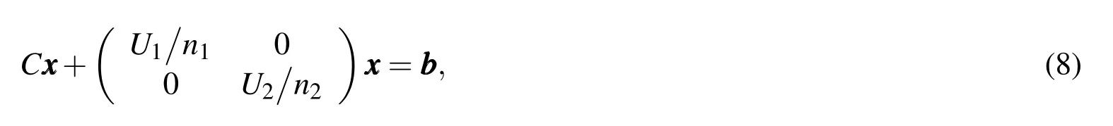
where the size of U matrices U1and U2are n1×n1and n2×n2,respectively(see Appendix B).Again,each row of the additional term represents the average of the unknown charges in the corresponding voxel-cluster.Finally,by rescaling the diagonal components to unity,the following simultaneous equations are obtained:

where the size of Cijandare ni× njand ni× 1,respectively.This technique is easily implemented in iterative solvers,is applicable to an arbitrary number of multiple clusters model,and has calculation cost of O(N).Note that if we analyze only the closed region problems,the field in each cluster can alternatively be solved with Eq.(7)by considering only the voxels in the cluster.However,Eq.(9)is available without any restriction.

2.4　Complexity of boundary element method with fast multipole method

The fast multipole method(FMM)[Rokhlin(1983),Greengard and Rokhlin(1997)]is one of the most famous algorithms that can be used to accelerate iterative solvers for simultaneous linear equations of BEM analysis[Bapat and Liu(2010),Wang and Yao(2011),Mallardo and Aliabadi(2012)].The FMM calculates interacting field among elements and the calculations are separated into two parts:(i)the direct interaction calculation of nearby elements,and(ii)the non-straightforward interaction calculation with multipole and local expansion coefficients.Here,we call the former and the latter as “near-part”and “far-part”calculations,respectively.The FMM is easily applied to the voxel-based BEM by regarding a cubic-shaped cluster of voxels,for example 6×6×6=63cubic voxels,as a leaf cell defined in the FMM algorithm.The details of the application of the FMM to the voxel-based IBEM are found in Hamada and Kobayashi(2006)and Hamada(2011,2013).Both the calculation time and the amount of memory required for solving=are expected to show O(N)dependency when using the Laplace kernel FMM.Besides,the number of surface elements N is expected to approximately exhibit O(D2)dependency,where D is the reciprocal of the voxel-side length,when the full size of an analyzed model is fixed.An example is explained in the next section.

3　Virtual-human model Duke

The IT’IS Foundation(www.itis.ethz.ch/vip)offers a series of anatomical virtual human models named the Virtual Population for research purposes.A subset of the Virtual Population with two adults and two children is named the Virtual Family.The adult male model of the Virtual Family is called Duke[Christ,Kainz,Hahn,Honegger,Zefferer,Neufeld,Rascher,Janka,Bautz,Chen,Kiefer,Schmitt,Hollenbach,Shen,Oberle,Szczerba,Kam,Guag,and Kuster(2010)](see Fig.1).Duke is 34 years old and composed of 77 types of tissues.Although these anatomical models are originally defined as triangular surface models,their direct utilization as surface models in general program codes is contractually restricted.However,we can derive voxel-version Duke models by using support software provided by the IT’IS Foundation.We can set the voxel-side length between 5.0 mm to 0.5 mm,and we can utilize voxel-version models in general codes.In addition,there are four types of voxel-version models provided in the distribution DVD(version 1.2)with the voxel-side length of 5.0 mm,2.0 mm,1.0 mm,and 0.5 mm.In this study,these four Duke models are used as a series of models having the same structural feature to examine the O(N)and O(D2)dependencies of the calculation time and the amount of memory of the voxel-based FMM-IBEM.

Figs.1(a)and 1(c)show the tissue numbers classified from 1 to 77 in a coronal slice of the model with 5.0 mm and 0.5 mm voxel-side lengths,respectively.The conductivities of tissues are assumed to be isotropic,and the values are assumed by mainly referring to the values in Hirata,Yamazaki,Hamada,Kamimura,Tarao,Wake,Suzuki,Hayashi,and Fujiwara(2010).Figs.1(b)and 1(d)show the calculatedand Fig.1(d)shows finer details of the field distribution compared with Fig.1(b).The number of voxels,number of boundary elements,and number of isolated clusters are summarized in Tab.1.The x,y,and z coordinates are defined as shown in Fig.1.The following can be observed in Tab.1:(i)the maximum number of total voxels exceeds 2.2 billion,and the number of voxels shows O(D3)dependencies;(ii)the maximum number of boundary elements reaches 61 million,and the number of elements approximately shows O(D2)dependency,which is approximately O(D2.1)for the voxel-version Duke models;(iii)a model is frequently composed of multiple voxel-clusters,thus,Eq.(9)should be used instead of Eq.(7)in such cases;and(iv)the number of clusters is non-predictable,thus it has to be counted by a subprogram developed for this purpose.

Figure 1:Tissue number and calculatedin Duke models.

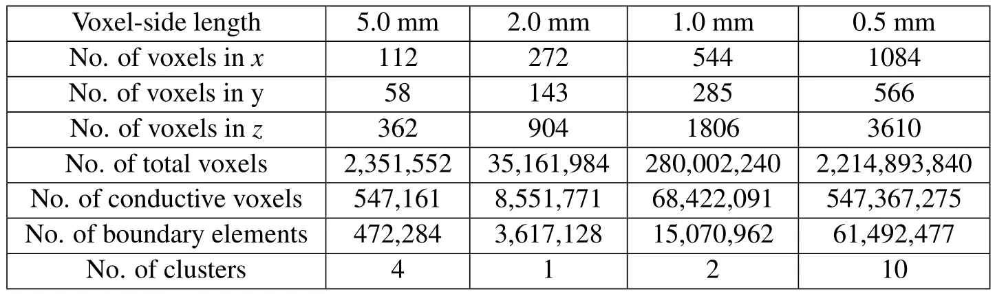
Table 1:The numbers of voxels,boundary elements,and isolated clusters.

4　Computing environment and settings

4.1　Computing environment

A personal computer running 64-bit Microsoft Windows 7 was used for the calculations.It had an Intel Core i7-4960X CPU(6 CPU cores,3.6 GHz)with 64 GiB of RAM.GPU acceleration[Hamada(2011,2013)]was not applied.The software was compiled with Intel Visual FORTRAN Composer XE 2013,and the number of OpenMP threads was set up to 12.

4.2　Settings for calculation

The applied homogeneous magnetic field B0(=B0k )was50-HzAC,1µT in strength,and parallel to the vertical axis.The vector potential was defined as A0=0.5B0(−y ii +x jjj),wherei,j,andkare the unit vectors parallel to the x,y,and z axes,respectively.

In the program code of the FMM algorithm,the order of the multipole and local expansions was set to ten.The translation algorithm that converts multipoleexpansion coefficients to local-expansion coefficients was a diagonal-form translation algorithm[Greengard and Rokhlin(1997)].The leaf-cell size that is defined as the voxel-cluster size was 53,63,or 73.The iterative solver used is the GBi-CGSTAB(s,L)[Tanio and Sugihara(2010)],where s=3 and L=2.This solver requires L(s+1)matrix-vector-product calculations before judging the convergence of the residual norm once.Here,we regard the number of matrix-vector products as the number of iteration steps.Thus,the convergence is judged every L(s+1)iteration steps.The convergence was decided when the relative residual norm became less than 10−6.However this criterion value was set to 10−10in subsection 5.1.

5　Results

5.1　Convergence performance of the linear equation solver

The convergence performance of the linear equation solver was investigated to confirm the validity of Eqs.(7)and(9).The voxel-side length of the Duke model used was 5.0 mm and the leaf-cell size was 63voxels.The model had one main-body cluster and three fragment clusters,with 547,150,8,2,and 1 voxels,respectively.Further,they had 472,234,34,10,and 6 boundary elements,respectively.

Fig.2(a)shows the result obtained when no measure is used to obtain a unique solution.The horizontal axis shows the iteration steps,and the residual norms,etc.are output once every L(s+1)=2(3+1)=8 steps.The upper figure shows the relative residual norm.The middle figure shows the absolute value of the sum of solution xiover the standard deviation of xi,which is an index of the deviation of total charges from zero.The lower figure shows the similar indices of clustercharges defined in each cluster.The index of total charge and indices of clustercharges exhibit intermittent increases and stagnation periods.The residual norm exhibits repeating decreases and stagnation periods,and the stagnation of residual norm appears to trigger increases in the charge indices.Empirically,increases in the charge indices tend to deteriorate the quality of the solution.The residual norm converges after 480 iterations.

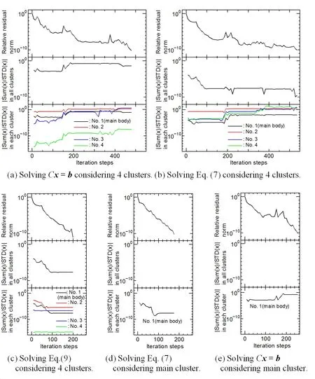
Figure 2:Comparison of convergence performance of the linear equation solver.

Fig.2(b)shows the result when Eq.(7),which constrains the total charge to zero,is used.The index of total charge decreases virtually to zero,as expected.However,the indices of cluster-charges still exhibit intermittent increases and stagnation periods.The residual norm exhibits repeating decreases and stagnation periods roughly in synchronization with the change of cluster-charge indices.The residual norm converges after 536 iterations.Fig.2(c)shows the result when using a kind of Eq.(9)that considers four clusters model,which constrains every cluster-charge to zero.All indices of charges decrease virtually to zero,as expected.The residual norm exhibits smooth convergence,and converges after 200 iterations.These results demonstrate that Eq.(9)is effective in achieving smooth convergence with the multiple clusters model.

Fig.2(d)shows the result obtained using Eq.(7)with a model containing only the main-body cluster.The residual norm converges after 176 iterations.These results are similar to those of Fig.2(c).Fig.2(e)shows the result obtained using no measure with a model containing only the main-body cluster.The index of total charge exhibits an intermittent increase and stagnation periods.The residual norm exhibits decreases and stagnation periods roughly in synchronization with the change of cluster-charge indices.The residual norm converges after 256 iterations.If we set the convergence criterion value to 10−6,it would require 208 iterations.Figs.2(d)and 2(e)demonstrate that Eq.(7)is effective in achieving smooth convergence with a single cluster model.

5.2　Calculation time and required amount of memory in the second stage

Calculation times and amount of memory required in the second stage are shown in Tab.2 and Figs.3,4,and 5.The numbers of required iteration steps,listed in Tab.2,are almost similar with the values ranging from 96 to 120.The solver took 6,587 s and 31.2 GiB in the finest model analysis with the setting of 73voxels in a leaf cell.

Figs.3(a)and 3(b)show the dependencies of one-step calculation time on N and D,respectively.Fig.3(a)shows the least square line of the fastest data at each N.The slope shows that the dependency is approximately O(N0.957).In a similar way,Fig.3(b)shows that the dependency is approximately O(D2.023).

Figs.4(a)and 4(b)show the dependencies of near-part and far-part calculation times on N,respectively.The dependencies are O(N0.847)and O(N1.07),respectively.The difference in these dependencies makes it necessary to adjust the number of voxels in a leaf cell to obtain the best performance as shown in Fig.3(a).

Fig.5 shows the amount of memory required in the second stage.The dependency is approximately O(N0.915).Thus,it is confirmed that the voxel-based IBEM ap-proximately exhibits the O(N1)and O(D2)dependencies of calculation times and amount of memory as expected.

Table 2:Calculation times and memory usage in the second stage.

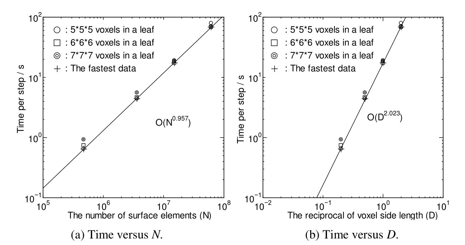
Figure 3:Dependencies of one-step calculation time on N and D in the second stage.

Figure 4:Dependencies of near-and far-part calculation times per iteration step on N in the second stage.

Figure 5:Dependency of memory in the second stage.

5.3　Calculation time and required amount of memory in the third stage

In the third stage,the static electric fields at all gravity centers of tissue voxels are calculated by using the FMM.The field strengths at all voxels,that is,not only tissue voxels but also air voxels,are output into a file to visualize the field distribution as shown in Fig.1.Calculation times and amount of memory required in the third stage are shown in Tab.3 and Fig.6.Figs.6(a)and 6(b)show the dependencies of the post-processing calculation time and the required amount of memory on N,respectively.The dependencies are O(N1.118)and O(N1.038),respectively.If N increased further,the dependencies would approach O(D3)=O(N1.5),which should be proportional to the number of voxels.However,such O(D3)dependencies were not observed,indicating that the proportional constant of the O(D2)part related to the FMM is larger than that of the O(D3)part at the present scale of problems.In addition,the amount of memory required in the postprocessing stage can be reduced by not storing the calculated value in arrays but directly writing them on a file,further reducing the proportional constant of the O(D3)part related to the amount of memory.

Table 3:Time and memory usage in the third stage.

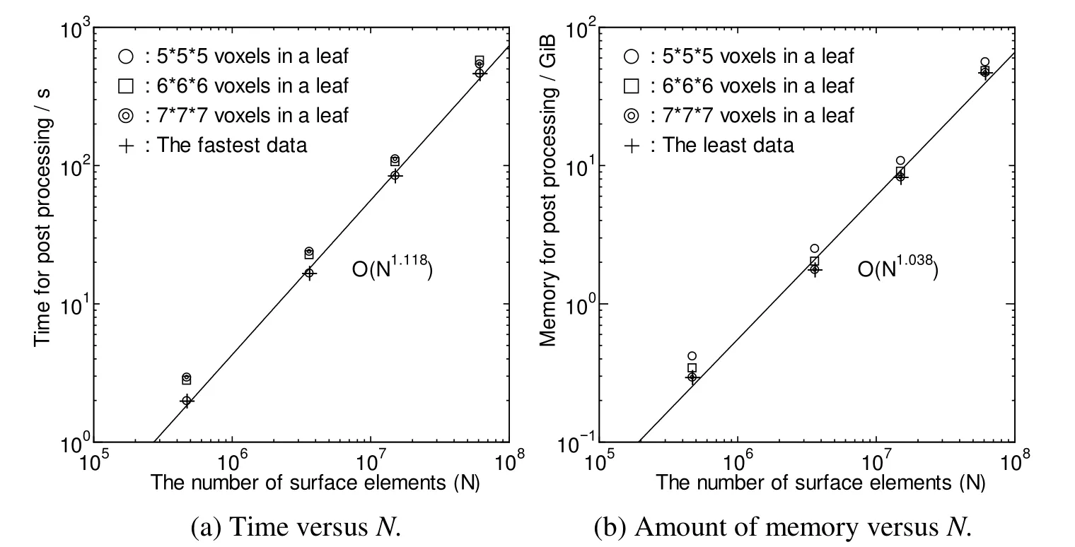
Figure 6:Dependencies of calculation time and amount of memory on N in the third stage.

6　Summary

A voxel-based FMM-IBEM was applied to analyze electrostatic fields induced by a 50-Hz homogeneous magnetic field in human anatomical voxel models.The analyzed models were voxel-version Duke models provided by the IT’IS Foundation.The voxel-side lengths were 5.0,2.0,1.0,and 0.5 mm.The linear equation solver took 6,587 s and 31.2 GiB on a personal computer for the finest model with 61 million boundary elements and 2.2 billion voxels.An important property of the voxelversion Duke models is that these models have different voxel sizes but the same structural feature.Taking advantage of this property,the O(N)and O(D2)dependencies of calculation times and amount of memory required for the voxel-based FMM-IBEM were con firmed.In addition,a technique to improve the convergence performance of the linear equation solver for the FMM-IBEM was proposed and its effectiveness was successfully demonstrated.

The results of this study suggest that the voxel-based BEM is an effective option in large-scale scientific computing environments.

Acknowledgement:This work was supported by JSPS KAKENHI Grant Number 25390153.

Bapat,M.S.;Liu,Y.J.(2010):A new adaptive algorithm for the fast multipole boundary element method.CMES:Computer Modeling in Engineering&Sciences,vol.58,no.2,pp.161–183.

Christ,A.;Kainz,W.;Hahn,E.G.;Honegger,K.;Zefferer,M.;Neufeld,E.;Rascher,W.;Janka,R.;Bautz,W.;Chen,J.;Kiefer,B.;Schmitt,P.;Hollenbach,H.P.;Shen,J.;Oberle,M.;Szczerba,D.;Kam,A.;Guag,J.W.;Kuster,N.(2010):The virtual family—Development of surface-based anatomical models of two adults and two children for dosimetric simulations.Phys.Med.Biol.,vol.55,no.2,pp.N23–N38.

Dawson,T.W.;Caputa,K.;Stuchly,M.A.(1997):In fluence of human model resolution on computed currents induced in organs by 60-Hz magnetic fields.Bioelectromagn.,vol.18,no.7,pp.478–490.

Dawson,T.W.;Caputa,K.;Stuchly,M.A.(1998):High-resolution organ dosimetry for human exposure to low-frequency electric fields.IEEE Trans.on Power Deliv.,vol.13,no.2,pp.366–373.

Greengard,L.;Rokhlin,V.(1997):A new version of the fast multipole method for the Laplace equation in three dimensions.Acta Numerica,vol.6,pp.229–269.

Hamada,S.(2011):GPU-accelerated indirect boundary element method for voxel model analyses with fast multipole method.Comput.Phys.Commun.,vol.182,pp.1162–1168.

Hamada,S.(2013):Performance comparison of three types of GPU-accelerated indirect boundary element method for voxel model analysis.Int.J.Numer.Model.,vol.26,pp.337–354.

Hamada,S.;Kobayashi,T.(2006):Analysis of electric field induced by ELF magnetic field utilizing fast-multipole surface-charge simulation method for voxel data.IEEJ Trans.FM,vol.126,pp.355–362(in Japanese)(translation(2008):Electr.Eng.Japan,vol.165,pp.1–10).

Hatada,T.;Sekino,M.;Ueno,S.(2005):Finite element method-based calculation of the theoretical limit of sensitivity for detecting weak magnetic fields in the human brain using magnetic-resonance imaging.J.Appl.Phys.,vol.97,no.10,10E109.

Hirata,A.;Yamazaki,K.;Hamada,S.;Kamimura,Y.;Tarao,H.;Wake,K.;Suzuki,Y.;Hayashi,N.;Fujiwara,O.(2010):Intercomparison of induced fields in Japanese male model for ELF magnetic field exposures:Effect of different computational methods and codes.Radiat.Protect.Dosim.,vol.138,no.3,pp.237–244.

Mallardo,V.;Aliabadi,M.H.(2012):An adaptive fast multipole approach to 2D wave propagation.CMES:Computer Modeling in Engineering&Sciences,vol.87,no.2,pp.77–96.

Rokhlin,V.(1983):Rapid solution of integral equations of classical potential theory.J.Comput.Phys.,vol.60,pp.187–207.

Tanio,M.;Sugihara,M.(2010):GBi-CGSTAB(s,L):IDR(s)with higher-order stabilization polynomials.Comput.Appl.Math.,vol.235,pp.765–784.

Wang,H.T.;Yao,Z.H.(2011):A fast multipole dual boundary element method for the three-dimensional crack problems.CMES:Computer Modeling in Engineering&Sciences,vol.72,no.2,pp.115–148.