Improved MPS-FE Fluid-Structure Interaction Coup led Method with MPS Polygon Wall Boundary M odel

N.Mitsume,S.Yoshimura,K.Murotani and T.Yamada

1　Introduction

Large facilities such as electric power plants built along coastal regions are vulnerable to tsunamis.The resulting damage to the equipment and instruments has the potential to cause catastrophic harm to people and devastate the locality.The Fukushima Daiichi nuclear disaster in Japan is a prominent example of this.It is economically impossible to completely mitigate the effects of disasters of extreme severity;however,damages and loss can be minimized through appropriate measures.

Regarding tsunami simulation,a great deal of research[Westerink,Luettich,Feyen,Atkinson,Dawson,Roberts,Powell,Dunion,Kubatko,and Pourtaheri(2008);Crespo,Gómez-Gesteira,and Dalrymple(2007)]has been conducted on the simulation of free surface flows using various numerical analysis methods.Although inundation areas and forces acting on structures can be modeled well by such simulations,the deformation and destruction of structures and the way in which water enters damaged structures are yet to be well understood.Clarifying these mechanisms w ill be of great value to disaster mitigation design.To this end,Fluid-Structure Interaction(FSI)analysis involving free surface flows is required.

The Finite Element Method(FEM)has been widely used for FSI analyses[Bazilevs,Calo,Hughes,and Zhang(2008);Takizawa and Tezduyar(2011)];however,in many of these applications,such as the vibration of airfoils,no free surfaces were present.In mesh-based methods including FEM,the fluid dynamics equations have a Eulerian basis,which means they have difficulty in dealing with a free surface.The level set method,the Volume Of Fluid(VOF)method,and the Arbitrary Lagrangian-Eulerian(ALE)method have been developed and applied for computing free surface flows and FSI problems involving free surfaces.Recently,the Particle Finite Element Method(PFEM)was developed[Oñate,Idelsohn,Pin,and Aubry(2004)]and used to solve challenging problems[Idelsohn,Marti,Limache,and Oñate(2008);Ryzhakov,Rossi,Idelsohn,and Oñate(2010);Oñate,Celigueta,Idelsohn,Salazar,and Suarez(2011)].This is an FEM-based full Lagrangian description of a fluid;therefore,it readily expresses free surfaces as the fluid domain boundaries.However,PFEM has a relatively high computational cost due to remeshing.

Mesh-free particle methods,such as the Smoothed Particle Hydrodynamics(SPH)method[Lucy(1977)]and the Moving Particle Simulation(MPS)method[Koshizuka and Oka(1996)],have also attracted attention.They discretize strong form equations and do not need node connectivity information.Based on a Lagrangian description of the fluid,they can deal with free surfaces easily and do not have the computational cost associated with mesh generation.Mesh-free particle methods have been applied to the dynamic analysis of solids and used to solve FSI problems[Antoci,Gallati,and Sibilla(2007);Rafiee and Thiagarajan(2009)].However,in contrast with the FEM automatically satisfying the Neumann boundary condition on the edge of a structure,mesh-free particle methods address the condition explicitly due to strong formulations.

In recent years,a coupling approach using the FEM in structures and mesh-free particle methods in fluids has been investigated for use in FSI analysis.The FEM/SPH coupling method[Lu,Wang,and Chong(2005)]was originally developed to compute blast and penetration analyses and was later applied to FSI analysis[Yang,Jones,and M cCue(2012)].

We developed the MPS-FE method[Mitsume,Yoshimura,Murotani,and Yamada(2014)]which adopts the MPS method for fluid computation involving free surfaces and the FEM for structure computation.The method combines the advantages of both methods and achieves efficiency and robustness as a result.However,the conventional MPS-FE method,in which MPS wall boundary particles and finite elements are overlapped in order to exchange information on fluid-structure interfaces,has difficulty in dealing with complex shaped fluid-structure boundaries,because the wall particles have to be set as uniform grids for accurate execution of the MPS.The result is cumbersome interpolation for the exchange of physical values and node-particle correspondence relation data for the interpolation are needed.Thus,the conventional MPS-FE method lacks versatility and reduces the software modularity.

In the present study,we improve the conventional MPS-FE method by using the MPS polygon wall boundary model[Harada,Koshizuka,and Shimazaki(2008);Yamada,Sakai,Mizutani,Koshizuka,Oochi,and Murozono(2011)]instead of the MPS wall particle model.Since the MPS polygon wall boundary model can express wall boundaries as plane polygons,the interface in the fluid computation now corresponds to that in the structure computation.This improvement overcomes the problems in the conventional method and improves versatility.

The outline of the present paper is as follows.The discretizations of the governing equations for the MPS method and the FEM are presented in Section 2 and Section 5,respectively.In Section 3,we describe the computation of the pressure on the polygons that is necessary to apply the polygon model to the MPS-FE computation,and discuss the accuracy and applicability in Section 4.Considering the pressure on the polygons,the formulation and algorithm of the improved MPS-FE is presented in Section 6.In order to verify the proposed method,an FSI problem involving a free surface is solved in Section 7.Conclusions complete the paper in Section 8.

2　MPS formulation for fluid dynamics

2.1　Governing equations

The Navier-Stokes equations and the continuity equation for aquasi-incompressible Newtonian fluid in a Lagrangian reference frame are given as follows:

whereρis the density of the fluid,vvvis the velocity vector,pis the pressure,νfis the kinetic viscosity,andis the gravitational acceleration vector.

2.2　MPS discretization

In the MPS discretization,the differential operators acting on a particleiare evaluated using the neighboring particlesjthat are located within an effective radiusre.Pirepresents the set of the neighboring particles of the particleias follows:

In this section,φijdenotesφj−φi,whereφrepresents a property of the particle.The neighboring particles are weighted using the weight function of their separation from particleIn the original MPS,the weight function is given as

To calculate the weighted average,a normalization factor termed the particle number density is de fined as

In the MPS method the fractional step algorithm is applied for time discretization,so each time step is divided into prediction and correction steps,as follows:

Hereis the intermediate velocity.The angle brackets〈〉indicate discretization by the MPS differential operators which are given as follows:

Heredis the number of dimensions andn0is the initial value of the particle number density given by Eq.(5).Similarly ton0,λ0is a quantity calculated for the initial geometry:

2.3　Pressure calculation

To calculate the correction step,Eq.(7),the pressure values in the next time steppn+1are required.For the pressure calculation,there are Sem i-Implicit MPS(SIMPS)methods[Koshizuka and Oka(1996)]in which the pressure Poisson equation is solved implicitly to determine the pressure values and an Explicit MPS(E-MPS)[Shakibaenia and Jin(2010)]method that assumes weak compressibility.

The present study employs the E-MPS method to compute the FSI with a free surface and is validated in Section 7.Assuming the weak compressibility of fluids,the explicit calculation of the pressure can be written as

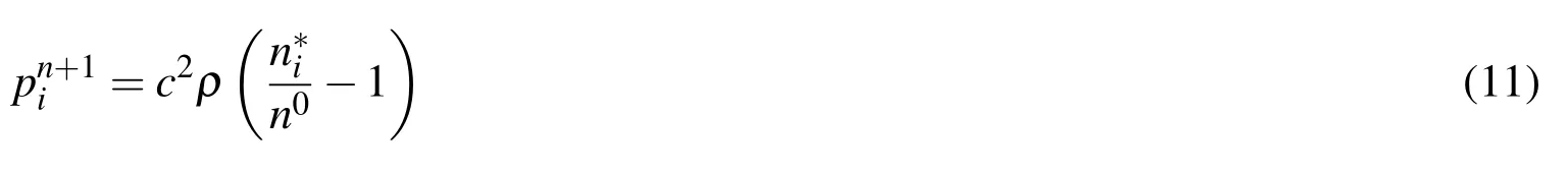
wherecis a parameter set arbitrarily to satisfy the conditions of stability and incompressibility.In addition,the E-MPS uses the following pressure gradient model instead of Eq.(8):

3　MPS polygon wall boundary model

In general,MPS computations use wall particles to model wall boundaries as illustrated in Fig.1.However,since the particles have to be set in uniform grids to correctly calculate the particle number density defined by Eq.(5),the wall particle model ineffectively simulates complex shaped boundaries.Harada et al.proposed the polygon wall boundary model[Harada,Koshizuka,and Shimazaki(2008)]which can express wall boundaries as plane polygons.By applying the polygon wall boundary model to an SI-MPS computation,they showed that the number of matrix elements in the pressure Poisson calculation and the computation time are reduced.A polygon wall boundary model applying the E-MPS has also been proposed[Yamada,Sakai,Mizutani,Koshizuka,Oochi,and Murozono(2011)].The differences between these two methods stem from the character of the pressure gradient term.In the present study,we use Yamada’s polygon wall boundary model because it has higher stability than Harada’s.

3.1　Wall weight function

To implement the polygon wall with no particles,the interpolation of the contributing part(green area at the right of Fig.1)within the particle number density computation is required.The wall weight function is de fined by the sum of the virtual wall particles’weights created inside the wall.Using the distance between the particle and the wallthe wall weight functionis de fined as

Figure 1:Wall particle model and polygon wall model

Within the neighboring particlesj∈Piof particlei,we de fine the fluid particles asj∈particleand the virtual wall particles asj∈wall.The particle number density Eq.(5)can be divided into the contributions of the fluid particles and the wall weight function as follows:

In the actual computation,the wall weight function is determined by the linear interpolation of values at the discrete distancewhich are calculated in advance of fluid computation.

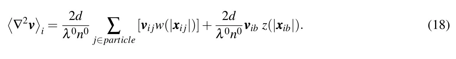
3.2　Viscosity term

The viscosity term discretized by the Laplacian model(9)is divided into fluid particle and polygon wall contributions:

Assuming that the velocity of the wallbis a constant valuewithin the effective radius of the particlei,the contributing region of the polygon wall can be deformed as follows:

Substituting the term into Eq.(15),the equation for the viscosity in the polygon wall model is derived as follows:

3.3　Pressure gradient term

As is the case with the viscosity term,the pressure gradient term is divided into the fluid particle and polygon wall contributions as follows:

As mentioned,the present study adopts Yamada’s pressure gradient model[Yamada,Sakai,Mizutani,Koshizuka,Oochi,and Murozono(2011)]:

3.4　Pressure on the polygon wall

The computation of the pressure on a polygon is described briefly in Yamada’s report,but is not clearly defined.Therefore,we formulate it here.

Let Wbbe the set of fluid particles that are influenced by the presence of the polygon wallb.The pressure on the polygon wall surface is the force exerted by the fluid particles per unit area.As shown in Fig.2,the force on the polygon wallbexerted by fluid particlesis the reaction to the sum of the pressure gradient forcesexerted by every particlejbelonging to the set Wbas follows:

wheremiis the fluid density andVis the volume occupied by a fluid particle.Assuming that all fluid particle radii are identical and the initial particle spacing isl0,the mass of each fluid particle can be calculated as.Thus,the pressure on the polygon wall can be computed as follows:

wheresbis the area of the polygonb.

Figure 2:The force on the polygon wall exerted by the fluid particles

4　Hydrostatic pressure calculation using MPS polygon wall boundary model

In order to verify the accuracy of the polygon wall boundary model with E-MPS and the pressure computation described by Eq.(24),we analyzed a hydrostatic pressure problem in a rectangular vessel and compared the result with the theoretical solution.The theoretical hydrostatic pressurepis given by the following equation:

wherehis the depth from the static water surface.

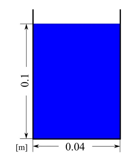
Figure 3:Hydrostatic pressure problem:initial con figuration

Table 1:Hydrostatic pressure problem:calculation parameters

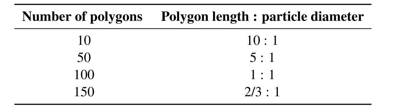
Table 2:Ratio of polygon length to particle diameter in each division

The initial con figuration of the hydrostatic pressure problem is shown in Fig.3.The rectangular vessel’s depth is 0.1[m]and the width is 0.04[m].We performed simulations with several numbers of polygons for the right hand wall and computed the pressures on the wall surfaces using Eq.(24).In E-MPS,weak compressibility causes vertical vibrations of the fluid surface.To reach the static state as soon as possible,we chose the highest value of viscosity that would not destabilize the computations.Figure 4,Fig.5,Fig.6,and Fig.7 show the average and standard variation of the pressure values from 40000th to 41000th steps into the simulation,with walls comprising 10,50,100,and 150 polygons,respectively.The ratio of the polygon length to the particle diameter is shown in Table 2.The average pressure values agree well with the theoretical values when the polygon length is large compared to the particle diameter,as shown in Fig.4 and Fig.5.In addition,since the pressure on the polygon is equivalent to the spatial average of the computed pressure,the pressure dispersion is reduced in the case of longer polygons.Several polygons have low pressure values in the cases where the polygon length is the same or shorter than the particle diameter,shown by Fig.6 and Fig.7.This occurs when polygons are not interacting with any particles,i.e.,Wb=/0 in Eq.(24).In this case,a non-smooth pressure distribution on the wall boundary results.In FSI simulations in particular,this in turn may cause unreason-ably high-order vibration modes in the structure and destabilize the computation;therefore,the polygon length should be set to more than twice the particle diameter for stability of computation.

Figure 4:Pressure on the right wall(10 polygons)

Figure 5:Pressure on the right wall(50 polygons)

Figure 6:Pressure on the right wall(100 polygons)

Figure 7:Pressure on the right wall(150 polygons)

5　FE formulation for structure dynamics

5.1　Governing equations for finite deformation

The virtual work equation of the total Lagrangian formulation with geometric nonlinearity is given as follows:

where Ωsis the structure dynamics domain with boundaryis the second Piola-Kirchhoff stress tensoris the Green-Lagrange strain tensor,ρis the density of the structure,andtttis the boundary traction in the reference con figuration.andin Eq.(26)are expressed using the deformation gradient tensoras follows:

whereis the second-order identity tensor andthe fourth-order elastic modulus tensor.In the present study,the Saint Venant-Kirchhoff model,which represents the linear relationship between the second Piola-Kirchhoff stress tensor and the Green-Lagrange strain tensor,was used.In this case,is expressed using the fourth-order identity tensor III and Lamé constantsλandµas follows:

5.2　Solution of non-linear problems

Because of the non-linear term in Eq.(26),non-linear solvers such as the New ton-Raphson method are required.Using the New ton-Raphson method,the discretized form of Eq.(26),

is solved iteratively as follows:

Herenis the time step,iis the iteration counter,is the external force vector,is the internal work vector,andandare the global mass matrix and the global tangent matrix,respectively,which are assembled from each element matrix.

5.3　Time integration scheme

The time integration scheme used in the present study is New mark’sβmethod:

In this study,we use the coefficient valuesβ=0.3025 andγ=0.6,which add numerical damping.This kind of damping has been frequently used as a stabilization technique for FSI computation[Ishihara and Yoshimura(2005);Bazilevs,Calo,Hughes,and Zhang(2008)].

6　Im proved MPS-FE fluid-structure interaction method

6.1　Fluid-structure interaction model

Figure 8:Conventional and improved MPS-FE

In the present study,the force on the polygon wallbexerted by the particlesjis described byIn addition,the point on the polygon surface from which a line perpendicular to the surface can extend to the particle is termed the effective position of the particle.Ind-dimensional computations,an effective position on a polygon wall can be expressed as a(d−1)-dimensional vectousing an arbitrary(d−1)-dimensional basis.Furthermore,there are shape functions in the normalized natural coordinateexpressed aon the surfaces of ad-dimensional solid element,whereis the number of nodes on the element surface.The effective positionof particlejexpressed in the normalized natural coordinate isThe point loads,which particlesj∈Wbexert on the polygonbare distributed as equivalent nodal forceson the nodeiusing the shape functionover the element surface as follows:

The pressure on the polygon described by Eq.(24)means the pressure values are constant.To replace Eq.(35)which expresses the fluid force as point loads,the equivalent nodal forces representing the pressure distributionare expressed as follows:

whereis the Jacobian matrix.If the pressure distribution on the polygonis computed using Eq.(24),the pressure values on the polygon are constant,,and detis equivalent to the area of the polygon.Hence,Eq.(37)can be rewritten as follows:

In this study,we used Eq.(38)for the computation of the problem presented in Section 7.

6.2　Partitioned coupling scheme

In the present study,the finite deformation FEM and the E-MPS method were used for FSI simulations.In this case,the fluid and structure computation time in a time step are quite different because the structure problem is solved implicitly and involves nonlinear iterations,whereas the fluid problem is solved explicitly.Additionally,the E-MPS computation requires a finer temporal resolution than the FEM.Therefore,the present study adopts a conventional serial staggered(CSS)scheme[Farhat and Lesoinne(2000)]as an FSI coupling strategy,which applies fluid computation to subcycling steps in order to set different values for the fluid time step Δtsand the structure time step Δtf.Furthermore,the pressures exerted on the structure are averaged overfluid subcycles in order to suppress the nonphysical pressure oscillation in the MPS.

The procedure at thenth time step is summarized below.

Determine the predicted values of displacemenand velocityfrom the previous values.

Perform the MPS calculationktimes and determine the averaged pressures exerted by the MPS wall boundary particlesas follows:

Convert the obtained pressuresinto the nodal equivalent forcesgiven by Eq.(38).

Perform the FEM calculation to obtain the updated displacementsand velocities

Figure 9:Presented weak coupling scheme based on CSS

7　Verification of the improved MPS-FE method

In order to verify the improved MPS-FE method,we solved the dam break problem with an elastic obstacle and compared the results with those obtained by other methods.

7.1　Simulation setup

Figure 10:Verification problem:initial con figuration(units:m)

The initial con figuration of the dam break problem with an elastic obstacle is illustrated in Fig.10.This problem was initially solved by[Walhorn,Kölke,Hübner,and Dinkler(2005)]using a space-time FEM and has since been investigated in other works[Idelsohn,Marti,Limache,and Oñate(2008);Ryzhakov,Rossi,Idelsohn,and Oñate(2010);Rafiee and Thiagarajan(2009);Kassiotis,Ibrahimbegovic,and Matthies(2010)].Calculation parameters are given in Table 3 and Table 4.

Table 3:Verification problem: fluid parameters

Table 4:Verification problem:structure parameters

7.2　Simulation result and comparison with other methods

Figure 11 shows the displacement of the upper-left corner of the elastic obstacle at each time step.In the figure,the result of the improved MPS-FE method is compared with that of the conventional MPS-FE method[Mitsume,Yoshimura,Murotani,and Yamada(2014)]and the particle FEM(PFEM)[Ryzhakov,Rossi,Idelsohn,and Oñate(2010)].Whereas the computation of the conventional MPSFE method in the previous study did not use any numerical damping for stabilization,the conventional MPS-FE computation shown here uses the same damping conditions as the improved MPS-FE method as described in Section 5.3.Snapshots of the simulation using the proposed method are shown in Fig.12.

Figure 11:Verification problem:comparison with other methods

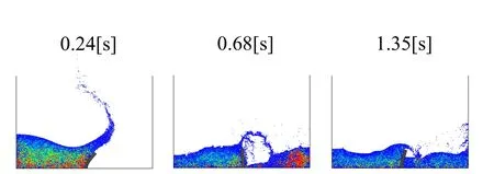
Figure 12:Verification problem:visualization of results

As shown in Fig.11,the improved MPS-FE result is in good agreement with the PFEM result.Although the conventional MPS-FE result is also in agreement with that of the PFEM to some degree,unnatural vibration after the initial deflection and a phase shift after 0.8[s]are observed.As mentioned previously,in the conventional MPS-FE approach,which uses the pressure values on the wall particles to exchange physical values,the forces on the fluid particles exerted by the structure are not consistent with the force on the structure computed by interpolation using the pressure on the wall particles.Since this inconsistency causes the fluid particles to exhibit unstable behavior near the fluid-structure interface,some fluid particles become too close or too far from the wall particles.The result is incorrect free surface determination and unreasonably high pressure values near the interface,leading to unnatural vibrations.The phase shift after 0.8[s]in the conventional MPS-FE method also comes from the inconsistency in exchanging physical values,which causes excessive decays in the energy.In converting the pressure on the wall particles to the equivalent nodal forces,energy is not conserved.In contrast,the improved MPS-FE method overcomes the problems in the transmission of force from the fluid to the structure by computing the force on the polygon wall directly using Eq.(24).

8　Conclusions

In the present paper,the improved MPS-FE method was proposed in which the MPS polygon wall boundary model is applied instead of using MPS wall particles,as were adopted in the conventional MPS-FE method.The computation method used to evaluate the pressure on the polygon wall was presented and the FSI model for the improved MPS-FE method was formulated.To verify the proposed method,the dam break problem with an elastic obstacle was solved.Comparing the result of the proposed method with that of the conventional method and PFEM indicated that the improved MPS-FE has adequate accuracy and higher stability and versatility.

Acknowledgement:The present paper was supported by the JSTCREST project"Development of a Numerical Library Based on Hierarchical Domain Decomposition for Post Petascale Simulation".

Antoci,C.;Gallati,M.;Sibilla,S.(2007):Numerical simulation of fluidstructure interaction by SPH.Computers and Structures,vol.85,pp.879–890.

Bazilevs,Y.;Calo,V.M.;Hughes,T.J.R.;Zhang,Y.(2008):Isogeometric fluid-structure interaction:theory,algorithms,and computations.Computational Mechanics,vol.43,pp.3–37.

Crespo,A.;Gómez-Gesteira,M.;Dalrymple,R.(2007):3D SPH Simulation of large waves mitigation with a dike.Journal of Hydraulic Research,vol.45,pp.631–642.

Farhat,C.;Lesoinne,M.(2000):Two efficient staggered algorithms for the serial and parallel solution of three-dimensional nonlinear transient aeroelastic problems.Computer Methods in Applied Mechanics and Engineering,vol.182,pp.499–515.

Harada,T.;Koshizuka,S.;Shimazaki,K.(2008):Improvement of wall calculation model for MPS method.Transactions of Japan Society for Computational Engineering and Science,,no.20080006.

Idelsohn,S.R.;Marti,J.;Limache,A.;Oñate,E.(2008):Unified lagrangian formulation for elastic solids and incompressible fluids:Application to fluid-structure interaction problems via the PFEM.Computer Methods in Applied Mechanics and Engineering,vol.197,pp.1762–1776.

Ishihara,D.;Yoshimura,S.(2005):A monolithic approach for interaction of incompressible viscous fluid and an elastic body based on fluid pressure Poisson equation.Computer Methods in Applied Mechanics and Engineering,vol.64,pp.163–203.

Kassiotis,C.;Ibrahimbegovic,A.;Matthies,H.(2010):Partitioned solution to fluid-structure interaction problem in application to free-surface flows.European Journal of Mechanics-B/Fluids,vol.29,pp.510–521.

Koshizuka,S.;Oka,Y.(1996):Moving-particle sem i-implicit method for fragmentation of incompressible fluid.Nuclear science and engineering,vol.123,pp.421–434.

Lu,Y.;Wang,Z.;Chong,K.(2005):A comparative study of buried structure in soil subjected to blast load using 2D and 3D numerical simulations.Soild Dynamics and Earthquake Engineering,vol.25,pp.275–288.

Lucy,L.B.(1977):A numerical approach to the testing of the fission hypothesis.Astronomical Journal,vol.82,pp.1013–1024.

Mitsume,N.;Yoshimura,S.;Murotani,K.;Yamada,T.(2014):MPS-FEM partitioned coupling approach for fluid-structure interaction with free surface flow.International Journal of Computational Methods,vol.11,no.4.1350101.

Oñate,E.;Celigueta,M.A.;Idelsohn,S.R.;Salazar,F.;Suarez,B.(2011):Possibilities of the particle finite element method for fluid-soil-structure interaction problems.Computational Mechanics,vol.48,pp.307–318.

Oñate,E.;Idelsohn,S.R.;Pin,F.D.;Aubry,R.(2004):The particle finite element method-an overview.International Journal of Computational Methods,vol.1,pp.267–307.

Rafiee,A.;Thiagarajan,K.P.(2009):An SPH projection method for simulating fluid-hypoelastic structure interaction.Computer Methods in Applied Mechanics and Engineering,vol.198,pp.2785–2795.

Ryzhakov,P.B.;Rossi,R.;Idelsohn,S.R.;Oñate,E.(2010):A monolithic Lagrangian approach for fluid-structure interaction problems.Computational Mechanics,vol.46,pp.883–899.

Shakibaenia,A.;Jin,Y.C.(2010):A weakly compressible MPS method for modeling of open-boundary free-surface flow.International Journal for Numerical Methods in Fluids,vol.63,pp.1208–1232.

Takizawa,K.;Tezduyar,T.E.(2011):Multiscale space-time fluid-structure interaction techniques.Computational Mechanics,vol.48,pp.247–267.

Walhorn,E.;Kölke,A.;Hübner,B.;Dinkler,D.(2005):Fluid-structure coupling within a monolithic model involving free surface flows.Computers and Structure,vol.83,pp.2100–2111.

Westerink,J.J.;Luettich,R.A.;Feyen,J.C.;Atkinson,J.H.;Dawson,C.;Roberts,H.J.;Powell,M.D.;Dunion,J.P.;Kubatko,E.J.;Pourtaheri,H.(2008):A basin-to channel-scale unstructured grid hurricane storm surge model applied to southern louisiana.Monthly Weather Review,vol.136,pp.833–864.

Yamada,Y.;Sakai,M.;Mizutani,S.;Koshizuka,S.;Oochi,M.;Murozono,K.(2011):Numerical simulation of three-dimensional free-surface flows with explicit moving particle simulation method.Transaction of the Atomic Energy Society of Japan,vol.10,pp.185–193.

Yang,Q.;Jones,V.;M cCue,L.(2012):Free-surface flow interactions with deformable structures using an SPH-FEM model.Ocean Engineering,vol.55,pp.136–147.