Boundary Layer Effect in Regularized Meshless Method for Laplace Equation

Weiwei Liand Wen Chen,2

1　Introduction

The regularized meshless method(RMM)belongs to the family of meshless boundary collocation methods[Young,Chen and Lee(2005)]and can be viewed as a regularized method of fundamental solutions(MFS)[Fairweather and Karageorghis(1998)]for the solution of certain boundary value problems.The method circumvents the fictitious boundary issue long perplexing the MFS[Ling,Opfer and Schaback(2006)]while being truly free of mesh and integral,and easy-to-program.Prior to this study,this method has been successfully applied to a variety of physical problems,such as potential[Young,Chen and Lee(2005)],exterior acoustics[Young,Chen and Lee(2006)],anti-plane shear[Chen,Chen and Kao(2008)],acoustic eigenvalue[Chen,Chen and Kao(2006)]and anti-plane piezoelectricity problems[Chen,Kao and Chen(2009)].Like to the other boundary-type numerical methods,the RMM,however,encounters a dramatic drop of solution accuracy at the region nearby the boundary,because of singularity of its double layer fundamental solutions.

Accurate evaluation of near-boundary solutions plays an important role in solving many engineering problems[Johnston and Elliott(2005)],such as contact[Aliabadi and Martin(2000)],inverse and sensitivity[Zhang,Rizzo and Rudolphi(1999)],thin-body[Luo,Liu and Berger(1998)],and crack problems[Dirgantara and Aliabadi(2000)],just to mention a few.In such cases,the calculation point is often placed very closely to,but not on,the physical boundary.Theoretically,the values of singular RMM kernel functions at these boundary-adjacent points are finite but not smooth at all.Nearby boundary,the kernels may have a sharp peak as the calculation point approaches closer to the boundary.Consequently,the kernels becomenearly singularand cannot be accurately calculated.

Inspired by the recent work on handling near singularity in the boundary element method and the singular boundary method[Gu,Chen and Zhang(2013);Gu,Chen and Zhang(2012)],this study applies an efficient nonlinear transformation[Johnston and Elliott(2005)],based on the sinh function,to remove or damp out the near singularity of the double layer fundamental solutions associated with the RMM.Compared with a straightforward implementation of the RMM,the transformed RMM proposed in this paper can improve the numerical accuracy and stability nearby boundary by several orders of magnitude in terms of relative errors.

A brief outline of the rest of this paper is as follows.The RMM formulation and its implementation for potential problems are presented in Section 2.And then Section 3 explains the principle of the nearly singular properties of the RMM formulation,and introduces the sinh transformation.In Section 4,the accuracy and validity of the transformed RMM are verified through three 2D potential examples,in which the solutions at interior points very close to the boundary are investigated in details.Finally,the conclusions and remarks are provided in Section5.

2　RMM formulation for 2D potential problems

Without a loss of generality,we consider the following Laplace problem:

subject to the following boundary conditions

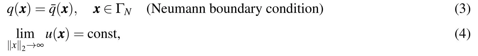
whereuis the potential field,Ω represents the computational domain,Γ=ΓD∪ΓN= ∂Ω denotes the boundary of the domain Ω,the barred quantities indicate the given values on the boundary.The fluxq(x)along the boundary ΓNis given by

wherendenotes the outward normal at the calculation point.In Eq.(4),‖x‖2represents the Euclidean distance,and const stands for a finite constant.It is noted that,for exterior problems,the potentialu(x)satisfies not only boundary conditions(2)and(3)but also the boundary condition(4)at infinity.

By using the radial basis function(RBF)method[Cheng,Young and Tsai(2000);Li,Lu,Hu and Cheng(2008);Liu(2007)],the solutionsu(x)andq(x)for interior problems can be approximated by:

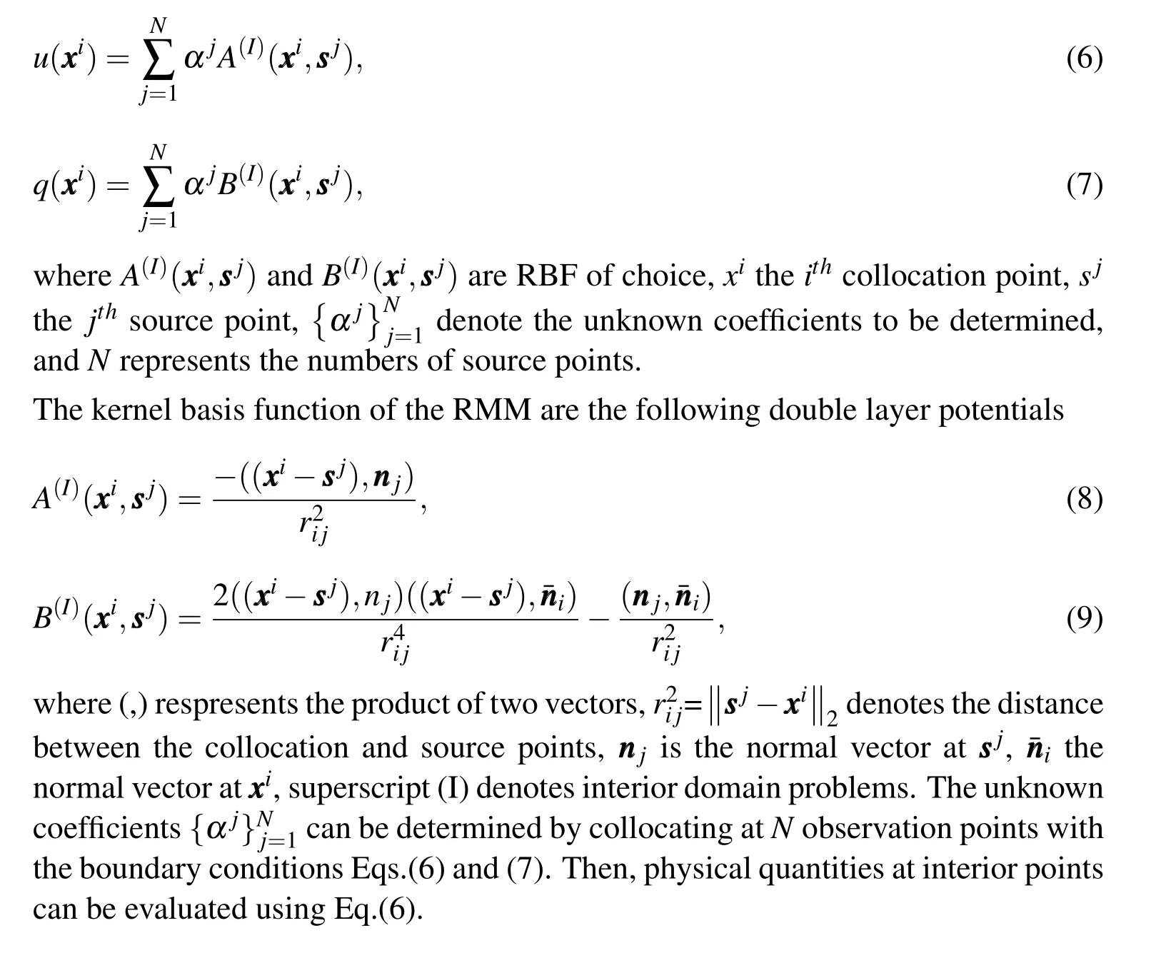
Similarly,the representation of the solution of exterior problem can be approximated as

where the superscript(E)denotes the exterior problems.

It is noted that,in the traditional MFS,the source points are placed on the fictitious boundary,for example,see Fig.1(a)and(b),outside the problem domain to avoid the singularity of kernel functions.However,the placement of fictitious boundary is largely based on experiences,especially for complex geometric and high dimensional problems[Berger and Karageorghis(2001);Fan,Chan,Kuo and Yeih(2012);Marin(2010)].Overcoming the abovementioned shortcoming,the source points of the RMM are distributed on the physical boundary,coincident with the collocation points,see Fig.1(c)and(d).

Figure 1:Problem sketch and nodes distribution using the conventional MFS and the RMM for interior and exterior problems:(a)interior problems(MFS),(b)exterior problems(MFS),(c)interior problems(RMM),and(d)exterior problems(RMM).

2.1　The RMM formulation for interior problems

When the collocation pointxiapproaches the source pointsj,the distance between these two nodes tends to zero,and the basis function kernels in Eqs.(6)and(7)present singular and hyper-singular.The RMM uses a subtracting and adding-back technique to remove the singularities of Eqs.(6)and(7)[Young,Chen and Lee(2005)].The diagonal elements of in fluence matrices can be derived from nullfield integral equations[Song and Chen(2009)]or the boundary integral equations(BIEs)[Sun,Chen and Zhang(2013)]at the domain point.The main results for 2D interior problems are summarized hereafter.

According to Ref.[Sun,Chen and Zhang(2013)],Eqs.(6)and(7)can be desingularized as follows:

whereljis half distance between the source points,and can be obtained by numerical integration,for example,the 8-points Gaussian quadrature.

Then the diagonal elements of the RMM interpolation matrix for interior problems can be derived by

2.2　The RMM formulation for exterior problems

For exterior problems,the diagonal elements can be determined via null- field integral equations[Song and Chen(2009)].Eqs.(10)and(11)can be regularized as follows:

The diagonal elements of the RMM interpolation matrix for exterior problems can be obtained by

By collocating BCs from Dirichlet boundary Eq.(2)and Neumann boundary Eq.(3)atNobservation points,the unknown coefficientscan be calculated by linear solvers.

A technique using the moment condition can be implemented in the RMM to remedy the wrong solution for the problem whose solution includes a constant potential[Chen,Fu and Wei(2009)].The potential at the pointyinside the domain is given by

with the constraint

wherexj∈ Γ,A(y,xj)=A(I)(y,xj)andA(y,xj)=A(E)(y,xj)correspond to interior or exterior problems,respectively.

3　Asinh transformation for nearly singular kernels in the RMM

From mathematical point of views,the RMM is equivalent to the indirect BEM(IBEM)and can be derived from a discretization formulation of the IBEM via a quadrature rule,as shown below

If the calculation pointis far away from the boundary,the numerical results by a straight forward application of the boundary integral equation(BIE)(22)will be sufficient to obtain accurate numerical results.However,if the calculationyyymoves closer to the boundary,the distance functionrapproaches to zero.Consequently,the BIE(22)will present nearly singularity.From the mathematical point of view,the integrand remains regular because it is finite at all points.However,instead of being smooth,the integrand may have a finite but very large gradient as the calculation point gets closer to the boundary.The whole integral,therefore,cannot accurately be calculated using the standard Gauss-quadrature.As a result,the RMM-expansion fails to yield reliable results nearby boundary.

As shown in Fig.2,we assume the calculation pointyyyis close to the boundary Γkcontaining the pointxk,then Eq.(22)can be rewritten as

whereukis defined as the nearly singular factor,which should be evaluated via special treatments.In this work,the nearly singular factorukis directly calculated as an average value of the kernel functions over Γkby

wherelkis half distance between the source nodes

Figure 2:A field point near the boundary.

In order to numerically calculate the above integral equation(24),the integral can be transformed and mapped onto the interval[1,1]in terms of some intrinsic coordinate ξ.If a quadratic boundary element is used,Eq.(24)can be rewritten as follows[Gu,Chen and Zhang(2013)]

where η ∈ [−1,1]stands for the position of the projection of the field point onto the element(see Fig.2),brepresents the shortest distance from the field point to the element,g(ξ)is a low order and non-negative polynomial,J(ξ)represents the Jacobian of the transformation from the quadratic boundary element to the interval[1,1],f(·)is a low-order polynomial which is a part of the kernel function.Further details can be found in Ref.[Gu,Chen and Zhang(2013)].

Due to the peaked nature of the integral, the above integral is difficult to numerically evaluate asb→0.To improve the accuracy of the numerical results in the RMM,a sinh transformation[Gu,Chen and Zhang(2013)]is used in this study

As mentioned above,g(t)function, and thus the function sinh2(k1t−k2)g(t)+1 in Eq.(29)is always greater than 1.Thus,an oscillating integrand is smoothed,and can now be accurately evaluated via the standard Gaussian quadrature,even if the value ofb,distance between boundary source and inner collocation points,is very small.

4　Numerical examples and discussions

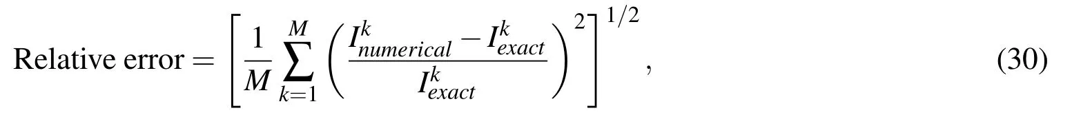
To verify the scheme developed above,three 2D potential problems are investigated in this section.The numerical results will be compared with exact solutions by the relative error defined below

4.1　Interior Dirichlet problem with gear wheel domains

First,we consider a bounded domain with gear wheel shape which is defined by

Problem sketch and the nodes distribution are depicted in Fig.3.The analytical solution is given by the global function

For the numerical implantation,N=1000source points are selected on the boundary.Tab.1 and 2 list the potential results at calculation pointsAandBin terms of the function of distancebfrom the boundary.The results using the original RMM are also given for a fair comparison.

As shown in Tab.1 and 2,when the calculation pointAandBare not very close to the boundary,the original RMM can obtain accurate results.However,ifAandBget closer to the boundary,i.e.,when the distancebis less than 1.0E-1,the RMM performs less accurate or even inaccurate.In contrast,results using the present transformed RMM are accurate and stable,even when the distancebis as small as 1.0E-6.This clearly shows that the transformed RMM performs much better than the original RMM in near-boundary regions.

Fig.4 shows the relative error curves of the potentials at point A and B withb=1.0E-6,against the number of boundary nodes.As illustrated in this figure,the transformed RMM converges quickly with an increasing number of boundary nodes even when the distance from the field point to the boundary is as small as 1.0E-6.

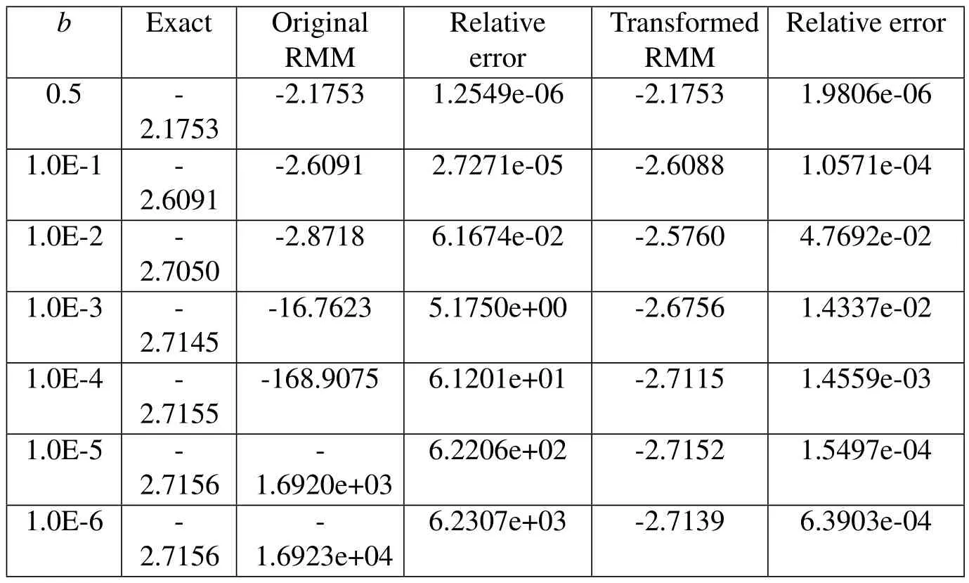
Table 2:Results of potential u at the calculation point B.

Figure 3:A bounded domain with gear wheel boundary shape.

Figure 4:Relative error curves of the transformed RMM.

4.2　Exterior Dirichlet problem with amoeba-like domain

Next,we consider an in finite domain with amoeba-like shape which is defined by

Figure 4 shows the pro file of the ameba-like shape boundary and the distribution of the source points.The symbols·and+represent the source points and computed points,respectively.

The exact solution is given by

To solve the problem numerically,N=1000 source points are placed on the boundary.The numerical solution accuracies are examined on a total ofM=90 calculation points with the off-boundary distanceb,as shown in Fig.5.

The relative error curves of the original and transformed RMMs are given in Fig.6 as functions of the off-boundary distanceb.We can observe from Fig.6 that the transformation technique increases a large degree of the accuracy near boundary solutions.It also illustrates that the relative errors decrease greatly,when the field point is far from the boundary,because the peak of integrand is becoming smooth.

Figure 5:The pro file of an in finite domain with amoeba-like boundary shape.

Figure 6:Relative error curves of potentials at interior points near the boundary using the transformed RMM and original RMM.

4.3　Multiply-connected domain with mixed boundary conditions

Finally,consider a multiply-connected domain problem.The shape of the domain and the nodes distribution are depicted in Fig.7.The symbols·and+represent source points and computation points,respectively.The boundary Γ is composed of the outer curve Γ1and the two inner curves Γ2∪Γ3as

where(nx1,nx2)is a unit normal vector,and the analytical solution is given byu(x1,x2)=sinx1coshx2.

Figure 7:Multiply-connected domain with mixed boundary conditions.

TakingN=800,80 and 40 source points on the outer boundary and two inner boundary,respectively.Selecting the same number of calculation points distributed inside the domain near the physical boundaries,whose distancebto the physical boundary varies from 0.5 to 1.0E-6.Fig.8 shows the relative error curves of potential results at the calculation points as functions of various values ofb.

Figure 8:Relative error curves of the potentials at interior points near the boundary using the transformed RMM and original RMM.

As shown in Fig.8,when the distancebis greater than 0.1,the results of the original RMM and the transformed RMM are both accurate.However,when the calculation points get closer to the boundary,the original RMM tends less accurate and stable.In stark contrast,the results using the proposed method remain accurate and numerically stable.It is also noting that when the distance to the boundary researches 1.0E-6,application of the transformation yields an improvement in relative error by about six orders of magnitude.As in the previous examples,the relative error of the proposed scheme is generally independent of the distancebfrom the boundary.

5　Conclusions

This paper introduces an efficient transformation technique to circumvent the boundarylayer effect associated with the RMM formulation.Compared with a straight forward implementation of the original RMM,the present transformed RMM produces an improvement in terms of relative error by several orders of magnitude.In general,the accuracy of the present RMM is less sensitive to the location of the nearly singular point and the distance between the field point and the boundary.The numerical experiments verify that accurate and stable results can be obtained using the proposed strategy even when the distance between the calculation point and the boundary is as small as1.0E-6.It is also observed from the foregoing numerical experiments that the proposed scheme performs numerically stable and its accuracy is largely independent of the distance from the calculated point to the boundary.

Acknowledgement:The work described in this paper was supported by,the Na-tional Science Funds for Distinguished Young Scholars of China(Grant No.11125208),the National Science Funds of China(Grant No.11372097),and the 111 Project(Grant No.B12032).

Aliabadi,M.H.;Martin,D.(2000):Boundary element hyper-singular formulation for elastoplastic contact problems.Int J Numer Methods Eng,vol.48,pp 995-1014.

Berger,J.R.;Karageorghis,A.(2001):The method of fundamental solutions for layered elastic materials.Eng Anal Bound Elem,vol.25,pp 877-886.

Chen,K.H.;Chen,J.T.;Kao,J.H.(2006):Regularized Meshless Method for Solving Acoustic Eigenproblem with Multiply-Connected Domain.comput Model in Eng Sci,vol.16,pp 27-39.

Chen,K.H.;Chen,J.T.;Kao,J.H.(2008):Regularized meshless method for antiplane shear problems with multiple inclusions.International Journal for Numerical Methods in Engineering,vol.73,pp 1251-1273.

Chen,K.H.;Kao,J.H.;Chen,J.T.(2009):Regularized meshless method for antiplane piezoelectricity problems with multiple inclusions.Cms-Computers Materials&Continua,vol.9,pp 253-279.

Chen,W.;Fu,Z.J.;Wei,X.(2009):Potential problems by singular boundary method satisfying moment condition.Comput Model in Eng Sci,vol.54,pp 65-85.

Cheng,A.H.D.;Young,D.L.;Tsai,C.C.(2000):Solution of Poisson’s equation by iterative DRBEM using compactly supported,positive definite radial basis function.Eng Anal Bound Elem,vol.24,pp 549-557.

Dirgantara,T.;Aliabadi,M.H.(2000):Crack growth analysis of plates loaded by bending and tension using dua lboundary element method.Int J Fract,vol.105,pp 27-47.

Fairweather,G.;Karageorghis,A.(1998):The method of fundamental solutions for elliptic boundary value problems.Adv Comput Math,vol.9,pp 69-95.

Fan,C.-M.;Chan,H.-F.;Kuo,C.-L.;Yeih,W.(2012):Numerical solutions of boundary detection problems using modified collocation Trefftz method and exponentially convergent scalar homotopy algorithm.Engineering Analysis with Boundary Elements,vol.36,pp 2-8.

Gu,Y.;Chen,W.;Zhang,C.(2013):The sinh transformation for evaluating nearly singular boundary element integrals over high-order geometry elements.Engineering Analysis with Boundary Elements,vol.37,pp 301-308.

Gu,Y.;Chen,W.;Zhang,J.(2012):Investigation on near-boundary solutions by singular boundary method.Engineering Analysis with Boundary Elements,vol.36,pp 1173-1182.

Johnston,P.R.;Elliott,D.(2005):A sinh transformation for evaluating nearly singular boundary element integrals.International Journal for Numerical Methods in Engineering,vol.62,pp 564-578.

Li,Z.C.;Lu,T.T.;Hu,H.Y.;Cheng,A.H.D.(2008):Trefftz and collocation methods.WIT Press.

Ling,L.;Opfer,R.;Schaback,R.(2006):Results on meshless collocation techniques.Engineering Analysis with Boundary Elements,vol.30,pp 247-253.

Liu,C.S.(2007):A modified Trefftz method for two-dimensional Laplace equation considering the domain’s characteristic length.Comput Model in Eng Sci,vol 21,pp 53-65.

Luo,J.F.;Liu,Y.J.;Berger,E.J.(1998):Analysis of two-dimensional thin structures(from micro-tonano-scales)using the boundary element method.Computational Mechanics,vol.22,pp 404-412.

Marin,L.(2010):Regularized method of fundamental solutions for boundary identification in two-dimensional isotropic linear elasticity.International Journal of Solids and Structures,vol.47,pp 3326-3340.

Song,R.C.;Chen,W.(2009):An investigation on the regularized meshless method for irregular domain problems.Comput Model in Eng Sci,vol.42,pp 59-70.

Sun,L.;Chen,W.;Zhang,C.(2013):A new formulation of regularized meshless method applied to interior and exterior anisotropic potential problems.Applied Mathematical Modelling,vol 37,pp 7452-7464.

Young,D.L.;Chen,K.H.;Lee,C.W.(2005): the potential problems with the potential problems with arbitrary domain.Journal of Computational Physics,vol.209,pp 290-321.

Young,D.L.;Chen,K.H.;Lee,C.W.(2006):Singular meshless method using double layer potentials for exterior acoustics.The Journal of the Acoustical Society of America,vol.119,pp.96.

Zhang,D.;Rizzo,F.J.;Rudolphi,T.J.(1999):Stress intensity sensitivities via hypersingular boundary integral equations.Computational Mechanics,vol.23,pp 389-396.