Can plasticity make spatial structure irrelevant in individual-tree models?

Oscar García

Can plasticity make spatial structure irrelevant in individual-tree models?

Oscar García

Background:Distance-dependent individual-tree models have commonly been found to add little predictive power to that of distance-independent ones.One possible reason is plasticity,the ability of trees to lean and to alter crown and root development to better occupy available growing space.Being able to redeploy foliage(and roots)into canopy gaps and less contested areas can diminish the importance of stem ground locations.

Growth and yield;Competition;Perfect plasticity approximation(PPA);siplab

Background

Distance-dependent individual-tree growth models,also known as spatially explicit individual-based models, have a long history in forestry(Dudek and Ek 1980; Newnham and Smith 1964;Reventlow 1879;Staebler 1951),and more recently have received considerable attention in plant ecology(Grimm 1999;Grimm and Railsback 2005;Wyszomirski 1983).In them,stem base or breast-height coordinates are used to compute indices that reflect the competitive status of each tree and predict growth and mortality.Although such models are valuable research tools,it has been generally found that tree locationscontributelittletopredictivepower,andinpractical forest management they have been almost entirely replaced by non-spatial approaches(Burkhart and Tomé 2012;Weiskittel et al.2011).

One possible reason for the insensitivity to stem location is plasticity,the ability of trees to lean and/or to adjust crown development so as to occupy less contested spaces(Longuetaud et al.2013;Muth and Bazzaz 2003;Rouvinen and Kuuluvainen 1997;Schröter et al. 2012;Seidel et al.2011;Stoll and Schmid 1998;Umeki 1995).Strigul et al.(2008)simulated forest stand development combining ideas from SORTIE(Pacala et al.1993) and from the canopy tessellation methods of Mitchell (1969,1975),but allowing for crown displacements as in Umeki(1995).They proposed aperfect plasticity approximation(PPA)as a limit where crowns are free to move so as to equalize competition intensity along their periphery.It was found that the simulation results were close to the PPA predictions,which do not depend on tree coordinates.

The main objective of this study was to complement the findings of Strigul et al.(2008),at the same time simplifying and generalizing aspects of that work. Their results are influenced by a number of specificassumptions and design choices,the importance of which are difficult to assess.Those include a space tessellation based on the intersection of crowns of a certain shape,allometric relationships linking tree dimensions to dbh,and particular growth functions.Here a general spatial individual-plant modelling framework implemented in thesiplabR package was used,testing several alternative assumptions about neighbouring tree interactions(García 2014).Simulations were run for three data sets with different species,tree sizes,and spatial structures.Unessential complications were avoided by using single-species even-aged stands,focusing instead on key mechanisms.Some extensions to mixed-species are discussed elsewhere(Lee and García,manuscript in preparation).

Spatial individual-tree models predict growth and mortality rates as functions of the target tree size,and of a competition or resource capture index that encapsulates neighbourhood effects.Observed correlations,however, do not imply causality,trees that grow faster because of genetic,microsite or other factors will be larger.Extrapolation of the individual variability in past growth rates, represented by current size,may be another reason for the prediction efficiency of aspatial models(García 2014). For the purposes of evaluating the effects of plasticity and spatial structure,we side-stepped the circular sizegrowth ambiguity issues by limiting the analysis to an index of effective resource capture(assimilation index, for short).Clearly,dependence or independence between the assimilation index and spatial structure implies the same for growth and survival.In addition,results will not depend on specific assumptions about growth relationships.

The next section describes the test data,the spatial individual-based models,perfect plasticity approximations,and the analysis of simulation output.Simulation results follow,focusing on how much of the assimilation variability is explained only by tree size(ignoring tree coordinates),with and without plasticity.The article continues with stand-level implications of perfect plasticity useful for whole-stand modelling and other applications,and ends with a Discussion and Conclusions. The Additional files 1 and 2 include computer code and additional details.

Methods

Data

Simulations were based on 3 plots from the Boreal Ecosystem-AtmosphereStudy(BOREAS,RichandFourni 1999).Theywereestablishedinunmanagednaturalstands in Manitoba and Saskatchewan,central Canada.Coordinates and diameter at breast height(dbh)were measured for all trees taller than 2 m on a 50×60 m area.Heights and crown dimensions were measured on a subsample, and estimated for all trees by regression on dbh.The stands were single species,approximately even aged,and situated on flat terrain.Plot characteristics are shown in Table 1;the crown base heights and crown widths are subsample averages.

García(2006)analyzed the same data and includes additional details.From two similar jack pine plots,only the one in the southern research site was used for this study. The data sets are included and documented in thesiplabpackage.

The jack pine attributes are intermediate between those oftheothertwoplots.Theaspentreesarelarger,andtheir densitysomewhatlower.Thesprucestandismuchdenser, with smaller trees and an irregular spatial pattern.Spatial distributions are shown in Figure 1(top row).

Models and simulation

Following Strigul et al.(2008),the model is most easily visualized through the physical crown space interactions of Mitchell’s TASS model(Mitchell 1975);generalizations are introduced later.In TASS,trees have a radially symmetrical potential crown shape with lateral crown expansion stopping at the points of contact,tessellating the plane on a horizontal projection(Figure 2a).The shapes move upward with height growth,modifying the tessellation,and possibly over-topping and eventually causing the death of the smaller trees.Light extinction produces a constant depth of live foliage,so that light interception and growth are essentially proportional to the horizontal area occupied by each tree.

Influencefunctions

It is often observed that crowns do not interlock,especially at higher latitudes,and a direct interpretation of the models of Mitchell(1975)and Strigul et al.(2008)is then unrealistic(Fish et al.2006;Goudie et al.2009). However,rather than as a crown surface,the shapes can be seen in a more abstract way as a shading potential or competitionintensityfunction,possiblyrepresentingboth above-ground and below-ground processes,which we call aninfluencefunction.Lightarrivesat variousangles,especially the important diffuse light radiation,so that the influence function is likely to extend somewhat beyond the physical crown limits.

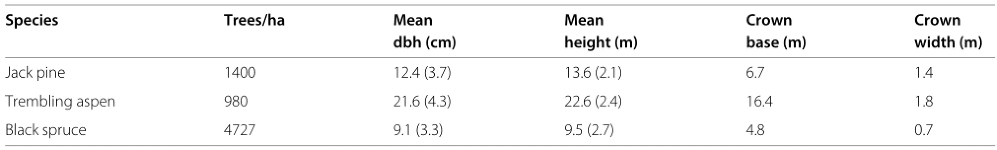
Table 1 Data statistics

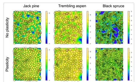
Figure 1 Tree spatial distributions for the 3 sample plots.Top:actual stem-base locations.Bottom:simulated crown displacements(simulation runs witha=1,α→∞,and distance-decreasing use efficiency).Circle diameters are proportional to tree height and zone of influence.Colour or shading follows influence function values.Trees in the 5 m border were excluded from displacements and from the analysis.

Regardless of interpretation,Gates et al.(1979)derived formsforacrownprofileorinfluencefunctionthatensure that the induced growing-space partition satisfies a number of reasonable properties.Their conditions,together with the assumption of shape preservation by upward movement through height growth(“gnomonic scaling”), imply that the surface height must follow the equation

whereHis tree height,Ris horizontal distance,andaandbare positive parameters(García 2014).Only positive values are used,otherwise the influence is taken as 0.The circlez=0 defines the treezone of influence(ZOI).

The simulations useda=1,which gives a cone,anda=2 that corresponds to a paraboloid of revolution.The pointed convex crown shapes used by Mitchell(1975)and Strigul et al.(2008)are intermediate between these two. Figure 2 was drawn using Eq.(1)witha=1.5.

The parameterbdetermines the shape slenderness, the ZOI extent,and the height of the function intersections between competing trees.The choice of values for the simulations is discussed later in Section‘Simulation parameters’.

Allotment

In TASS and in Strigul et al.(2008),the horizontal space is subdivided on an exclusive basis,with the tree having the largest influence function value taking all the resource (e.g.,light)available at each point.Competition is completelyasymmetric.Alessextremealternativeistoassume that the resource is somehow shared among trees where their ZOIs overlap.Siplabimplements a general allotment rule where at each point(or pixel)a tree with influence function valuezicaptures a proportion

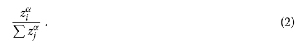
The sum is over all the trees(or over all trees with positive influence at that point),and the parameterαis ameasure of local competition asymmetry.Withα=1 resource capture is directly proportional toz.In the limitα→ 0 capture is fully symmetric,the same for all competing trees independently ofz.Forα→ ∞one has the TASStessellationwherethelargestztakesall.Simulations were run withα→∞and withα=1.

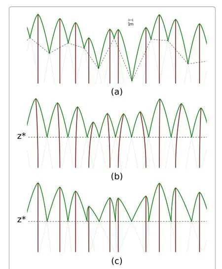
Figure 2 Plasticity mechanisms that tend to equalize the competition pressure from the tree neighbours.The curves represent potential crown profiles,or more generally,shading potential or competitive strength(influence function).Dashed lines join neighbour contact points.(a)No plasticity.(b)Leaning.(c) Differential branch growth.A combination of these mechanisms can be expected,in addition to a redistribution of foliage density. Produced withAsymptote(http://asymptote.org)usinga=1.5 in Eq.(1).

Efficiency

As mentioned before,the area allocated to a tree can be used as a summary of the effect of the neighbours on its development.For a givenα,the values of(2)are spatiallyintegrated,assumingauniformresourcedistribution with one unit per unit area.Siplabdiscretizes these calculations,a 10-cm square pixel was used.More generally, the integration can be weighted by anefficiency function, to produce an effective resource capture or assimilation index reflecting contributions that diminish with distance from the tree location.An efficiency function of the same formastheinfluencefunctionwasused,scaledbyitsvalue at the origin∶

This efficiency is 1 at the tree location,and decreases to 0 at the edge of the ZOI.The tessellations of Mitchell(1975) and Strigul et al.(2008)correspond to the special caseα→∞with a flat efficiency function.

Plasticity

With plasticity,phototropism induces a displacement toward areas where more light is available.Leaning of the stem in the direction of canopy gaps is common (Figure 2b).Differential branch growth(Figure 2c)and redistribution of foliage density can also be important. In most cases a combination of all these mechanisms is likely.Either way,the result is a more even resource allocation and less dependence on the basal stem locations. Note that plasticity makes the height of the crown contact or influence function intersection points more uniform.Below ground,roots can follow similar asymmetric patterns(Brisson and Reynolds 1994).

To simulate plasticity,tree coordinates were iteratively displaced to the centroid of the tree efficiency-weighted pixel resource captures.This tends to equalize competitive pressure on opposite sides,in the spirit of Umeki (1995)and Strigul et al.(2008).Iterations terminated when all coordinates changed by less than 5 cm.To prevent unlimited drifting,limits on the maximum displacement from the original tree position were enforced (Section‘Simulation parameters’).Distortions due to the absence of competitors beyond the plot boundaries were limited by excluding a 5 m border from coordinate changes and from the results(Figure 1).

This approach does not distort the influence profiles as in Figure 2c.However,it can be seen that only the vertical change in cross-sectional area near the contact height is important.Another simplification is that,as in Strigul et al.(2008),crowns are displaced but the cross-sections remain circular.In reality,in many tree species horizontal crown shape distortion can add significantly to the spatial regularization of the canopy,although crown displacements still seem to be the main factor(Longuetaud et al.2013).

Perfect plasticity

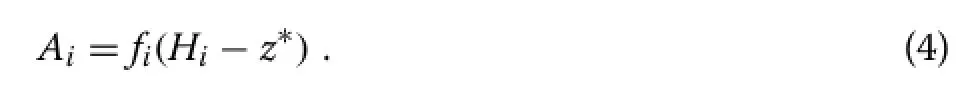
In theperfect plasticity approximation(PPA)of Strigul et al.(2008),plasticity causes all the crown contact points to be at a common heightz∗(Figure 2).Consider a general influence function,where the horizontal cross-sectional area for treeiis some functionfiof the distance from the top.Then,forα→∞,the area captured by the tree is

Assuming full canopy closure(z∗＞0),these areas must add up to the total stand area,so that the mean area is

whereNis the number of trees per unit area.This equation determines the contact levelz∗;a numerical solution is generally necessary.

In the models of Strigul et al.(2008)all tree dimensions for a tree species are fixed functions of dbh,andfivaries with species and dbh.With gnomonic scalingfiis sizeinvariant,and for Eq.(1)is

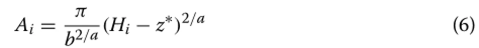
ifHi≥z∗,otherwiseAi=0.The parameters can be species-dependent.

From equations(5)and(6),

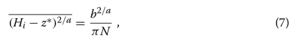
provided that all trees are taller thanz∗.Explicit expressions forz∗can be obtained fora=1 anda=2.In the paraboloida=2,the tree areaAiis a linear function ofHi,and eq.(7)reduces to

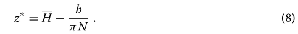
In the conea=1 the function is quadratic,and

whereσ2is the height variance,giving

With the weighting of eq.(3),the effective resource capture or assimilation indexcan be obtained by integration over annular differentials of area 2πrdr∶

giving

Some additional relationships are derived in Section‘Stand-level implications’.

Finding an explicit assimilation PPA for non-tessellation models(α＜∞)seems more complicated.In any case, resource capture under perfect plasticity,and the consequentpredictedgrowthandmortality,dependontreesize and stand density but not on spatial coordinates.

Simulation parameters

It remains to choose values for the parameterbin eq.(1), and limits for the ZOI displacements.

The stands have closed canopies,signalled by a rising canopy base.Influence intersection heights should therefore lie mostly above the average green crown level.It seemed reasonable to choosebso that the PPA intersections are about 2 m above the crown base,for a foliage depth of approximately 2 m(Mitchell 1975).Values thus obtained from equations(8)-(9)and Table 1 are shown in Table 2.Other values ofbgave qualitatively similar simulation results.

With regards to displacement limits,the plasticity literature usually reports means for the horizontal distances between crown centroid and stem base,often as relative displacements(displacement divided by mean crown radius),but maximum values are less common.Muth and Bazzaz(2003)show relative displacements less than 1 for mixed hardwoods.In old-growth European beech, Schröter et al.(2012)found a maximum displacement of 6.26 m.Longuetaud et al.(2013)gave relative displacements of up to 7.68 in mixed broadleaves.In Scots pine, Vacchiano et al.(2011)calculated stand means between 1.0 and 3.9 m across 4 sites in the Alps.Figure five of Gatziolis et al.(2010)shows horizontal deviations between surveyed stem base and LiDAR-assessed tree top exceeding 10 m in both conifers and hardwoods,although some of that may be due to measurement error.

Besides crown displacement,foliage distribution also affects the influence function,and the contribution of crownshapedistortion(Longuetaudetal.2013)isignored in the model.Based on this information,for the main results the algorithm total ZOI displacement was limited by a seemingly conservative upper bound of 3 m in all cases.To assess the effects of this parameter,also partial results with more restrictive bounds of 1.5 m for pine and 1 m for spruce will be shown(the spruce narrower crowns and perhaps their closer spacing might justify the smaller bound;aspen exhibits more stem leaning than conifers).

Analysis

We are interested in to what extent allowing for plasticity in the simulations diminishes the effect of spatial structure.In other words,how good is a perfect plasticity approximation,which assumes that assimilation indices depend only on tree size.To that effect,assimilation indiceswere analyzedbothin the absenceofplasticity,i.e., with the original tree coordinates,and after convergence of the ZOI displacement algorithm.

Table 2 Values of the parameterbused in the simulations

As a direct visual evaluation,the spread in scattergrams of assimilation index over tree height was examined,for the various model variants and data sets.The simulated values were compared to the theoretical tessellation PPA relationships of Section‘Perfect plasticity’.As a numerical summary,the r-squared from a quadratic polynomial regression indicated the proportion of variance accounted for by tree size alone.

Also of interest are the differences in total resource capture(sum of the assimilation indices).Values per unit area and tree averages were calculated.

In a tessellation,some smaller trees may be completely over-topped,receiving no resources.The centroiddriven ZOI displacement algorithm ignores these trees, affecting total resource utilization(this is not the case withα＜∞).The proportion of such trees is shown in the results.The proportion of trees where the displacement was constrained by the bounds of Section‘Simulation parameters’wasalso computed.This indicates to what extent approaching the PPA was limited by those assumptions.

The trend toward a more regular spatial distribution under plasticity was assessed with the Clark and Evans aggregation index,calculated withspatstat(Baddeley and Turner 2005)using the default Donnelly edge correction (Rouvinen and Kuuluvainen 1997;Schröter et al.2012). Theindexis1fora“random”(Poisson)pattern,valuesless than 1 indicate clustering,while more uniform spacings produce indices greater than 1.

Results and discussion

Simulation

Simulation results are shown graphically in Figures 3,4,5, and numerical summaries are given in Table 3.Note that the simple iterative algorithm generally progresses toward more balanced competition,but there is no guaranteed convergence to any sort of optimum;anomalies can occur.

Figure 3 Simulation results for jack pine.Without plasticity,much of the assimilation variability is due to the spatial structure of tree locations. Plasticity reduces the effect of tree coordinates,so that the variability is largely explained by tree height.Curves are the tessellation(α→∞) assimilation PPA.It is seen that the approximation is satisfactory in that case,but clearly it is not appropriate forα=1.

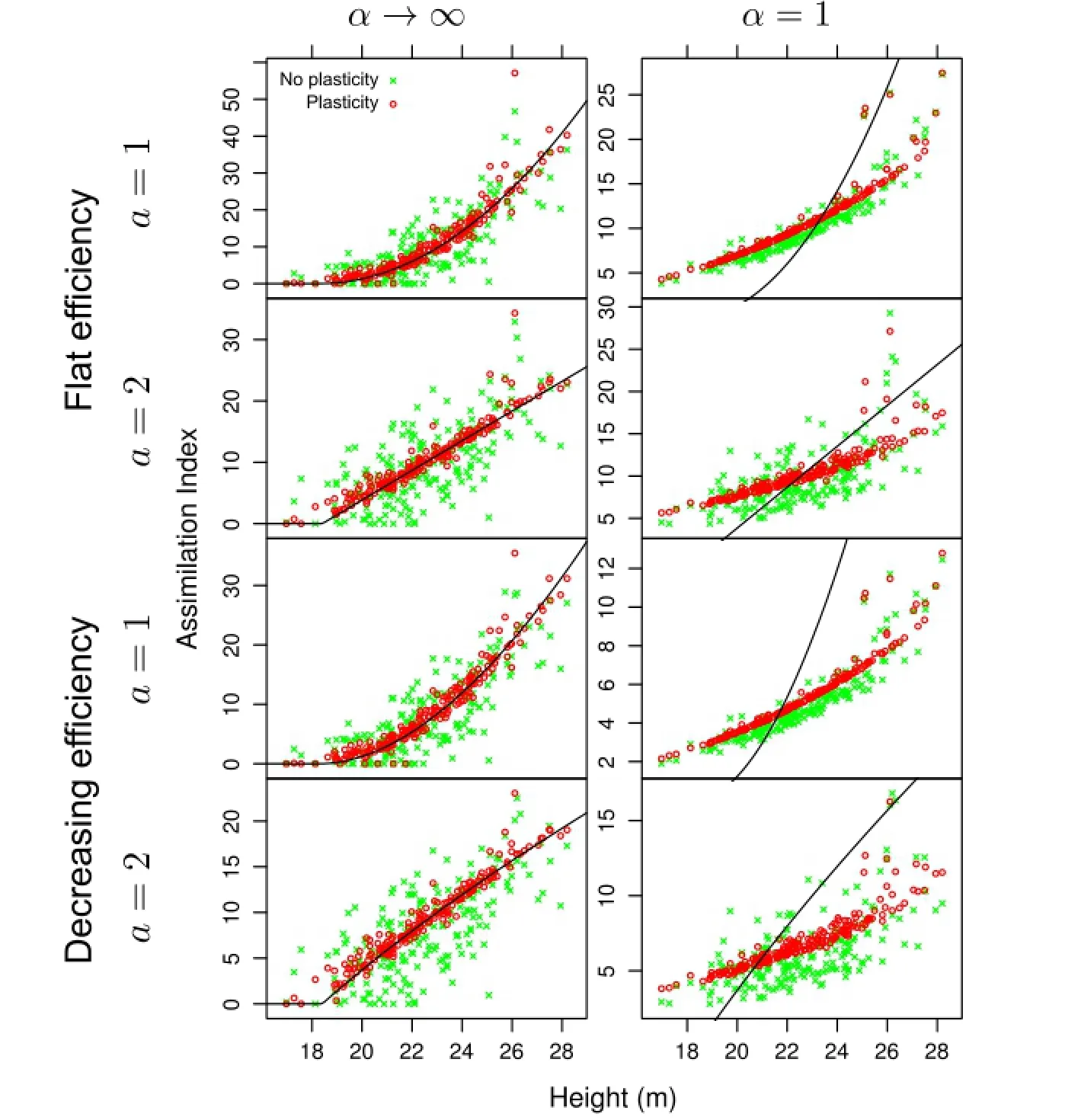
Figure 4 Simulation results for trembling aspen(see the legend of Figure 3).Outliers correspond to trees close to a large gap.

Simulated plasticity resulted in good relationships between assimilation indices and tree size,in most instances explaining over 90%of the variance as indicated by the regressionR2.That is,less than 10%of the variability can be attributed to spatial structure.The assimilation PPA works well for the tessellation models on which it is based(α→ ∞),but the relationships forα=1 are substantially different.

The Clark-Evans aggregation index indicates clustering of the stem coordinates.Plasticity moves the ZOIs into less occupied areas,tending to a more regular pattern, See also Figure 1.For the same reason,the total resource capture(or mean assimilation)increases,although perhaps not as much as might have been expected.The outliers with high assimilation indices in the aspen graphs of Figure 4 correspond to trees near the large gap on the bottom-right corner of Figure 1.

In the tessellation models,trees that are underneath the influence functions of other trees have zero assimilation,and do not participate in the displacements unless movement of their competitors changes their circumstances.That can be seen in the graphs,and in the rows labelled“%with assimilation 0”in Table 3.These trees are relatively more numerous in the more heterogeneous spruce stand.Withα＜∞all trees receive some resources.

About half of the pine and spruce trees,and 1/4 of the aspens,are constrained by the 3 m displacement bound at the last iteration.This and the visually tighter relationships for the aspen suggest that relaxing this bound would decrease further the importance of spatiality.To examine the effects of more severe constraints,simulations were run with displacement limits of 1.5 m for pine and 1 m for spruce.ResultsareshowninTable4fordistance-weighted efficiency.As expected,theR2decreased,although size still accounts for much of the variation.

Stand-level implications

A number of global relationships can be derived from the perfect plasticity approximation.These can be useful for canopy depth prediction,distribution modelling,and to develop whole-stand models for complex stands.

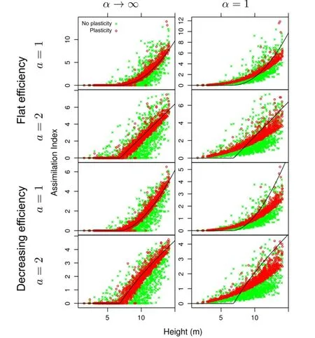
Figure 5 Simulation results for black spruce(see the legend of Figure 3).In this denser and more heterogeneous stand the effect of plasticity is weaker.

Canopydepth

With perfect plasticity,a tree crown length equals the distance from the top to the contact levelz∗,plus the depthdof the foliage layer∶

andz∗is related to stand densityNas described in Section‘Perfect plasticity’.The mean canopy depth is

From eq.(7),for the crown profiles or influence functions of eq.(1)

As a first approximation,ignoring the height variability gives

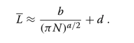
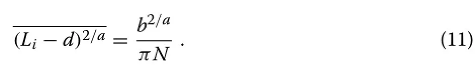
A second order approximation can be obtained applying the delta method(a 2nd order Taylor expansion aroundL)on the left-hand side of(11),leading to

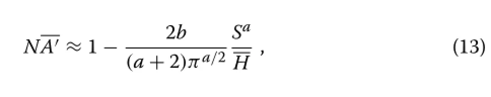
whereC=σ/Lis the coefficient of variation of the crown lengths.Eitherway,assumingthatCisrelativelystable,the mean canopy depth is approximately linear in 1/Na/2,or in terms of the average spacingS=approximately linear inSa.In the special casea=1 eq.(9)gives an exact relationship that is only slightly nonlinear,while fora=2 equations(8)and(12)coincide.

Brown(1962)and Valentine et al.(1994)used a similar argument with equal-sized conical crowns,but assuming that the crown base coincided withz∗,to conclude thatshould be proportional toS.Beekhuis(1965)and Valentine et al.(2013)found that including an intercept ina linear regression gave better results for pine plantation data.That agrees with eq.(12)fora= 1(Beekhuis’canopy depth was based on stand top height instead of mean height,so that his intercept includes the difference between those height measures).

Table 3 Simulation results,maximum displacement 3m

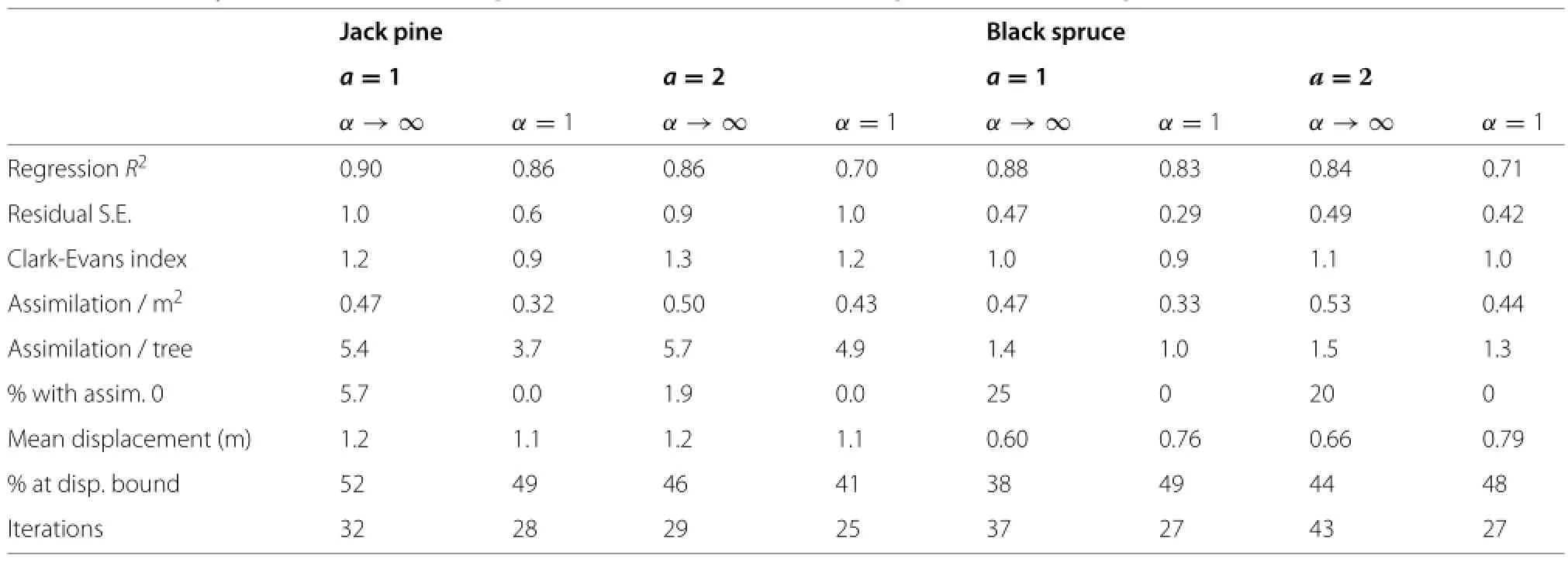
Table 4 Plasticity simulations with displacement bounds of 1.5 m for pine and 1 m for spruce

A nonlinear least-squares regression with Beekhuis’ data,in metric units,gives= 3.67+3.77S0.742orL=6.26+1.97S,with the exponent not significantly different from 1(p= 0.456).A similar analysis with the grouped summaries from Table two of Amateis and Burkhart(2012),excluding the age 5 data which might not have reached canopy closure,gives=2.30+0.854S1.27or=1.54+1.41S,again with the exponent not significantly different from 1(p=0.429).The linear regression is similar to those of Valentine et al.(2013)for individual trees from the same experiment.These observations support a value ofa≈1,at least for conifers.

Distributions

Perfect plasticity makes growth and mortality independent of tree locations,they only depend on tree size and stand density.The state of a stand is then fully characterized by a size distribution andN.In a discrete approximation,individual-based aspatial models can then simulate the development of a finite sample of trees,as in the traditional distance-independent individual-tree growth and yield models(Burkhart and Tomé 2012;Weiskittel et al.2011).

Strigul et al.(2008)calculated the evolution of a continuous size distribution with a partial differential equation(PDE)known as the McKendrick or von Foerster equation.It extends the classical Liouville equationtoincludemortalityandrecruitment(Picardand Franc 2004).Introducing stochastic elements would produce the Fokker-Planck(or Kolmogorov forward)PDE. Stochastic differential equations are a sometimes advantageous alternative representation.

Another possibility is to avoid PDEs by describing the state through the distribution moments instead of a continuous function.In general,this would require an infinite sequence of equations,one for the rate of change of each moment.Theproblemis solvedbymoment closure methods,which ignore higher moments or approximate them as functions of lower-order moments(e.g.,Milner et al. 2011;Murrell et al.2004).

Most models have used a simple scalar measure of tree size,usually dbh or basal area.A biologically meaningful tree description,however,requires at least two variables such as height and volume or biomass,a two-dimensional size vector(García 2014).In principle,the methods above can be applied to vectors,although that has rarely been done.

It should be recognized that the size-dependent growth or mortality relationships apply only within a stand.Large dominant trees tend to grow faster than the stand average, but at the landscape level large trees may correspond to older stands with lower growth rates.Hierarchical statistical methods should give better results than the common practiceoffittingsimpleregressionstodatagatheredfrom different stands.

Aspatiallyuniformresourceavailabilityisalsoassumed. This is appropriate for light,but nutrients and moisture vary and tend to be spatially correlated.In fact, for these data sets neighbouring tree sizes were found to be positively correlated,instead of the negative correlation predicted by spatial competition models,or of the independence assumed when using distributions (García 2006).In aspen,clonal vegetative propagation adds to the positive size correlations through spatial clustering of genotypes and growth rates.

As mentioned in the Introduction,a growth-size correlation may not be due to large size causing faster growth,but to the fact that faster-growing trees are larger.Specially with diameter-driven models and undermanagement or natural disturbances,this statistical confounding can be problematic(García 2014).

Whole-stand

Production can be expected to be approximately proportionaltoeffectiveresourcecapture,sothatthereisinterest inthetotalassimilationorassimilationperunitarea.With a flat efficiency function,assimilation corresponds to the area allocated to the tree,and with full canopy closure the total is independent of stand density and spatial structure(although it can change with stand age or height,and withsiteproductivity).Ifuseefficiencydecreaseswithdistance,however,stand assimilation and biomass or volume growth should decrease with increasing average spacing (García 1990).

Under the PPA withα→∞and ignoring size variability,equations(10)and(7)give the following approximation for the assimilation per unit area∶

withS=being the average spacing.As in Section‘Canopy depth’,the delta method can be used to produce a more accurate approximation of the same form.This is similar to moment closure(Section‘Distributions’),retaining only the first moment.García (1990)found in radiata pine that gross volume increment per hectare,adjusted for site quality,decreased linearly withS,pointing again toa≈1.

If this is still approximately true withα＜∞is an open question.

Conclusions

These simulations are static,representing one point in time,instead of simulating stand development over long periodsoftimeasinStriguletal.(2008).However,dynamically the plasticity adjustments correspond tofast variablesthat act on much shorter time scales than tree growth,leading approximately to a dynamic equilibrium. Dispensing with the details of full growth,mortality and regeneration models allows for more general inferences, appropriate to the time horizons typically considered in growth and yield prediction.This might not be sufficient for studying succession mechanisms,including natural regeneration and changes in species composition over several centuries(Strigul et al.2008).

Ignoring crown distortion underestimates the effectiveness of plasticity in reducing the effects of spatial pattern. With circular cross-sections it is not possible to achieve in three dimensions the idealized equalizing of inter-tree competition pressures suggested by Figure 2.That would require the crown or influence function width to vary withazimuth,leadingtoirregularcross-sectionssimilarto those commonly observed in practice(Longuetaud et al. 2013).Therefore,one would expect tighter relationships than those shown in Figures 3,4,5,unless the 3 m bound on displacements turns out to be far too high.

Intuition and experimental results suggest that the simplecentroid-chasingalgorithmtendstothePPA,although that is not mathematically proven.Even so,the algorithm does not necessarily always converge to a“best”solution, and improvements might be possible.At a more fundamental level,it is not entirely obvious why the uniformz∗of Strigul et al.(2008)might be biologically optimal or desirable.In fact,it can be shown that deviations from it can increase the total effective resource capture by the stand,so it may not be strategically optimal at the population level in the sense of Parker and Smith(1990).Balancing competitive pressure on all sides seems however a reasonable tree-level tactic.

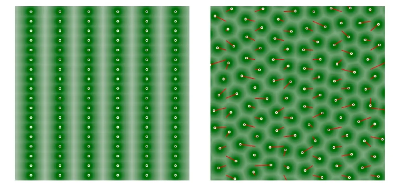
Figure6 Rectangularplanting.Left:no plasticity,crowns centred on the rectangular planting pattern.Right:plasticity simulated with the centroidchasing algorithm,crowns are displaced into less contested spaces.Shading indicates effective resource capture,line segments show the displacementofthecrowncentroidfromthestembaselocations.Treesat1.5×4.5mspacing,Hi=14m,a=1,b=3.5,α→∞,efficiencyweighting.

Thesimulationssupportedthehypothesisthatplasticity causes assimilation indices,and hence growth andmortality,to be affected much less by tree location than by tree size.The degree of spatial independence varied among the test stands,presumably mainly in relation to the regularity of the spatial pattern.The plastic capabilities of the trees,represented by the bounds on maximum displacement,can be important in the more irregular stands.These conclusions were robust,mostly insensitive to assumptions about influence function shape,competition asymmetry,or resource use efficiency.The PPA assimilation-size relationships derived from tessellation models were not appropriate with less extreme asymmetry(α=1);it would be interesting to find correct explicit equations for that case.

Plasticity can also help to explain the insensitivity to spacing rectangularity in forest plantations.It has been observed that planting pattern has little or no effect on tree sizes,mortality,or yield(e.g.,Amateis and Burkhart 2012).A simulation of equal-sized trees on a 1∶3 rectangular spacing(Figure 6)showed that plasticity produced tree growing areas indistinguishable from those arising from square spacing(a small random coordinate perturbation was used to get the algorithm started).With plasticity the total assimilation was 15%higher than without plasticity.

Fertility and other spatial correlations,and growth-size statistical confounding,are additional reasons for the generally small contribution of tree coordinates to growth predictions(Section‘Distributions’).More research on these topics is needed.

It appears that for spatial patterns that are not too irregular,and for sufficiently plastic tree species,there is little to be gained by including spatial structure in growth and yield forecasting models.However,spatial modelling is likely to be still important in relation to severe disturbances and gap dynamics,and their effects on natural regeneration and succession.Difficulties with distance-independent and other distribution-based models(Section‘Distributions’)make whole-stand modelling approaches attractive.Extensions of the PPA and similar approximations to multiple species,and to cohorts in uneven-aged forests,can produce whole-stand level equations suitable for complex stands.

Additional files

Additional file 1:Rcode and details.

Additional file 2:Animations of the plasticity simulation algorithm. ZIP file with PDF and GIF formats:a1infeff:aspen,a=1,α=∞, efficiency weighting;p1infeff:pine,a=1,α=∞,efficiency weighting; p11eff:pine,a=1,α=1,efficiency weighting;rectAnim:1:3 rectangular spacing.

Competing interests

The author declares that he has no competing interests.

Acknowledgements

Useful comments from anonymous reviewers of various versions of the manuscript contributed to improve the text.The work was funded through the FRBC/West Fraser Endowed Chair in Forest Growth and Yield,University of Northern British Columbia.

Received:29 May 2014 Accepted:25 July 2014

Published:12 August 2012

Amateis RL,Burkhart HE(2012)Rotation-age results from a loblolly pine spacing trial.South J Appl Forestry 36(1):11-18.doi:10.5849/sjaf.10-038

Baddeley A,Turner R(2005)Spatstat:an R package for analyzing spatial point patterns.J Stat Softw 12(6):1-42.http://www.jstatsoft.org/v12/i06.

Beekhuis J(1965)Crown depth of radiata pine in relation to stand density and height.N Z J Forestry 10(1):43-61.http://www.nzjf.org/free_issues/ NZJF10_1_1965/4B04540F-06D3-4A4C-B26B-0BD3510F36EE.pdf.

Brisson J,Reynolds JF(1994)The effect of neighbors on root distribution in a creosotebush(Larreatridentata)population.Ecology 75:1693-1702. doi:10.2307/1939629

Brown GS(1962)The importance of stand density in pruning prescriptions. Empire Forestry Rev 41(3):246-257

Burkhart HE,Tomé M(2012)Modeling forest trees and stands.Springer, Dordrecht,The Netherlands.doi:10.1007/978-90-481-3170-9

Dudek A,Ek AR(1980)A bibliography of worldwide literature on individual tree based forest stand growth models.Staff Paper Series Number 12, University of Minnesota,Department of Forest Resources

Fish H,Lieffers VJ,Silins U,Hall RJ(2006)Crown shyness in lodgepole pine stands of varying stand height,density,and site index in the upper foothills of Alberta.Can J Forest Res 36(9):2104-2111. doi:10.1139/x06-107

García O(1990)Growth of thinned and pruned stands.In:James RN,Tarlton GL (eds)New Approaches to Spacing and Thinning in Plantation Forestry: Proceedings of a IUFRO Symposium,10-14 April 1989,pp.84-97,Rotorua, New Zealand,Ministry of Forestry,FRI Bulletin No.151.http://web.unbc.ca/ garcia/publ/thinned.pdf.

García O(2014)A generic approach to spatial individual-based modelling and simulation of plant communities.Int J Math Comput Forestry Nat Res Sci 6(1):36-47.http://www.mcfns.com/index.php/Journal/article/view/6_36.

García O(2006)Scale and spatial structure effects on tree size distributions: Implications for growth and yield modelling.Can J Forest Res 36(11):2983-2993.doi:10.1139/x06-116

Gates DJ,O’Connor AJ,Westcott M(1979)Partitioning the union of disks in plant competition models.Proc R Soc Lond A 367:59-79. doi:10.1098/rspa.1979.0076

Gatziolis D,Fried JS,Monleon VS(2010)Challenges to estimating tree height via LiDAR in closed-canopy forests:A parable from Western Oregon.Forest Sci 56(2):139-155

Goudie JW,Polsson KR,Ott PK(2009)An empirical model of crown shyness for lodgepole pine(Pinuscontortavar.latifolia[Engl.]Critch.)in British Columbia. Forest Ecol Manag 257(1):321-331.doi:10.1016/j.foreco.2008.09.005

Grimm V(1999)Ten years of individual-based modelling in ecology:what have we learned and what could we learn in the future?Ecol Model 115(2-3):129-148.doi:10.1016/S0304-3800(98)00188-4

Grimm V,Railsback SF(2005)Individual-based modeling and ecology. Princeton University Press,Princeton and Oxford

Longuetaud F,Piboule A,Wernsdörfer H,Collet C(2013)Crown plasticity reduces inter-tree competition in a mixed broadleaved forest.Eur J Forest Res:1-14.doi:10.1007/s10342-013-0699-9

Milner P,Gillespie CS,Wilkinson DJ(2011)Moment closure approximations for stochastic kinetic models with rational rate laws.Math Biosci 231(2):99-104.doi:10.1016/j.mbs.2011.02.006

Mitchell KJ(1969)Simulation of the growth of even-aged stands of white spruce.School of Forestry Bulletin No.75,Yale University,New Haven,CT

Mitchell,KJ(1975)Dynamics and simulated yield of Douglas-fir.Forest Science Monograph 17,Society of American Foresters,Washington,D.C

Muth CC,Bazzaz FA(2003)Tree canopy displacement and neighborhood interactions.Can J Forest Res 33(7):1323-1330.doi:10.1139/x03-045

Murrell DJ,Dieckmann U,Law R(2004)On moment closures for population dynamics in continuous space.J Theor Biol 229(3):421-432. doi:10.1016/j.jtbi.2004.04.013

Newnham RM,Smith JHG(1964)Development and testing of stand models for Douglas-fir and lodgepole pine.Forestry Chron 40:494-504. doi:10.5558/tfc40494-4

Pacala SW,Canham CD,Silander JJA(1993)Forest models defined by field measurements:I.The design of a northeastem forest simulator.Can J Forest Res 23:1980-1988.doi:10.1038/348027a0

Parker GA,Smith JM(1990)Optimality theory in evolutionary biology.Nature 348(6296):27-33.doi:10.1038/348027a0

Picard N,Franc A(2004)Approximating spatial interactions in a model of forest dynamics.FBMIS 1:91-103.http://cms1.gre.ac.uk/conferences/iufro/fbmis/ A/4_1_PicardN_1.pdf.

Reventlow CDF(1879)A Treatise of Forestry.Society of Forest History, Horsholm,Denmark(English translation,1960)

Rich PM,Fournier R(1999)BOREAS TE-23 Map Plot Data,Data set available on-line(http://www.daac.ornl.gov)from OakRidgeNational Laboratory Distributed Active Archive Center,Oak Ridge,Tennessee,USA

Rouvinen S,Kuuluvainen T(1997)Structure and asymmetry of tree crowns in relation to local competition in a natural mature Scots pine forest.Can J Forest Res 27(6):890-902.doi:10.1139/x97-012

Schröter M,Härdtle W,Oheimb G(2012)Crown plasticity and neighborhood interactions of European beech(FagussylvaticaL.)in an old-growth forest. Eur J Forest Res 131(3):787-798.doi:10.1007/s10342-011-0552-y

Seidel D,Leuschner C,Müller A,Krause B(2011)Crown plasticity in mixed forests-Quantifying asymmetry as a measure of competition using terrestrial laser scanning.Forest Ecol Manage 261(11):2123-2132. doi:10.1016/j.foreco.2011.03.008

Staebler GR(1951)Growth and spacing in an even-aged stand of Douglas-fir. Master’s thesis,School of Natural Resources,University of Michigan

Stoll P,Schmid B(1998)Plant foraging and dynamic competition between branches ofPinussylvestrisin contrasting light environments.J Ecol 86(6):934-945.doi:10.1046/j.1365-2745.1998.00313.x

Strigul N,Pristinski D,Purves D,Dushoff J,Pacala S(2008)Scaling from trees to forests:tractable macroscopic equations for forest dynamics.Ecol Monogr 78(4):523-545.doi:10.1890/08-0082.1

Umeki K(1995)A comparison of crown asymmetry betweenPiceaabiesandBetulamaximowicziana.Can J Forest Res 25(11):1876-1880. doi:10.1139/x95-202.

Vacchiano G,Castagneri D,Meloni F,Lingua E,Motta R(2011)Point pattern analysis of crown-to-crown interactions in mountain forests.Procedia Environ Sci 7(0):269-274.doi:10.1016/j.proenv.2011.07.047

Valentine HT,Ludlow AR,Furnival GM(1994)Modeling crown rise in even-aged stands of Sitka spruce or loblolly pine.Forest Ecol Manage 69(1-3):189-197.doi:10.1016/0378-1127(94)90228-3

Valentine HT,Amateis RL,Gove JH,Mäkelä A(2013)Crown-rise and crown-length dynamics:application to loblolly pine.Forestry 86(3):371-375.doi:10.1093/forestry/cpt007

Weiskittel AR,Hann DW,Kershaw JAJ,Vanclay JK(2011)Forest growth and yield modeling.Wiley-Blackwell,Chichester,UK

Wyszomirski T(1983)Simulation model of the growth of competing individuals of a plant population.Ekologia Polska 31(1):73-92

Cite this article as:García:Can plasticity make spatial structure irrelevant in individual-tree models?ForestEcosystems2014 1:16.

Submit your manuscript to a SpringerOpen journal and benef i t from:

▶ Convenient online submission

▶ Rigorous peer review

▶ Immediate publication on acceptance

▶ Open access: articles freely available online

▶ High visibility within the fi eld

▶ Retaining the copyright to your article

Submit your next manuscript at ▶ springeropen.com

10.1186/s40663-014-0016-1

Correspondence:garcia@unbc.ca

University of Northern British Columbia,3333 University Way,V2N 4Z9 Prince George,BC,Canada

©2014 García;licensee Springer.This is an Open Access article distributed under the terms of the Creative Commons Attribution License(http://creativecommons.org/licenses/by/4.0),which permits unrestricted use,distribution,and reproduction in any medium,provided the original work is properly credited.

Methods:Plasticity was simulated for 3 intensively measured forest stands,to see to what extent and under what conditions the allocation of resources(e.g.,light)to the individual trees depended on their ground coordinates.The data came from 50×60 m stem-mapped plots in natural monospecific stands of jack pine,trembling aspen and black spruce from central Canada.Explicit perfect-plasticity equations were derived for tessellation-type models.

Results:Qualitatively similar simulation results were obtained under a variety of modelling assumptions.The effects of plasticity varied somewhat with stand uniformity and with assumed plasticity limits and other factors.Stand-level implications for canopy depth,distribution modelling and total productivity were examined.

Conclusions:Generally,under what seem like conservative maximum plasticity constraints,spatial structure accounted for less than 10%of the variance in resource allocation.The perfect-plasticity equations approximated well the simulation results from tessellation models,but not those from models with less extreme competition asymmetry. Whole-stand perfect plasticity approximations seem an attractive alternative to individual-tree models.