Numerical investigation of drag force on flow through circular array of cylinders*

YU Ling-Hui (余凌晖), ZHAN Jie-min (詹杰民)

Department of Applied Mechanics and Engineering, SunYat Sen University, Guangzhou 510275, China,

E-mail: sysuylh@163.com

LI Yok-sheung (李毓湘)

Department of Civil and Environmental Engineering, The Hong Kong Polytechnic University, Hong Kong, China

Numerical investigation of drag force on flow through circular array of cylinders*

YU Ling-Hui (余凌晖), ZHAN Jie-min (詹杰民)

Department of Applied Mechanics and Engineering, SunYat Sen University, Guangzhou 510275, China,

E-mail: sysuylh@163.com

LI Yok-sheung (李毓湘)

Department of Civil and Environmental Engineering, The Hong Kong Polytechnic University, Hong Kong, China

(Received March 5, 2013, Revised March 19, 2013)

A 2-D model for flow through a circular patch with an array of vertical circular cylinders in a channel is established using the Navier-Stokes equations with a hybrid RANS/LES turbulence model–the Scale Adaptive Simulation (SAS) model. The applicability of the model is first validated by test cases where experimental data are available for comparison with the computed results. It is verified that the present model can predict well the average velocity and turbulence structure. The drag force and drag coefficient are then calculated using the present model for a number of cases with different solid volume fractions, cylinder Reynolds numbers and patch diameters. It is shown that the drag coefficient increases with increasing solid volume fraction, but decreases with increasing Reynolds number. However, the drag coefficient is independent of the diameter of circular batch when the solid volume fraction and Reynolds number are kept constant.

Scale Adaptive Simulation (SAS), circular patch, drag coefficient

Introduction

Vegetation plays a key role in the sustainable development of aquatic environment. It provides habitat and food to various species of aquatic animals. Vegetation can also change the distribution of flow velocity, turbulence structure, and deposition and erosion patterns, offering protection to shorelines and riverbeds.

Laboratory experiments on flow through vegetation were carried out by Ghisalberti and Nepf[1], and Nezu and Onitsuka[2]. Those studies have shown the complex flow patterns, turbulence and diffusion in flows through vegetation. In those experiments, vegetation elements are simplified as rigid cylinders or blades.

There are many numerical studies on such vegetated flows. Two approaches are commonly used to simulate the flows. The first approach considers flow around each vegetation element and is called the multi-body model. Each vegetation element is commonly simplified as a circular cylinder and the no-slip boundary condition is applied on the surface of each cylinder. Stoesser et al.[3]presented an LES model to fully resolve the turbulent flow through a matrix of cylinders by a high-resolution grid. Okamoto and Nezu[4]also conducted 3-D numerical simulation of flow through a group of rigid strip plates. The multibody model could reproduce both the large-scale (vegetation zone) and small-scale (vegetation element) turbulence structures. The second approach uses a simplified model, which is called the porous model. In this model, individual vegetation elements are not considered. The vegetation zone is only treated as a porous zone, with the resistance of the vegetation taking into account by adding a drag force term to the momentum equations when the flow passes through the vegetation zone. Su and Li[5]proposed a k-l LES model to simulate the turbulent flow in partly vegetated open channel. The porous model does not require fine grids, but can only predict the large-scale motion. However, the computed results may be adequate for engineering design purposes.

In the porous model, the effect of vegetation is only determined by the strength of the resistance source used in the momentum equations and hence the determination of a suitable drag coefficient Cdis the key to a successful simulation. For a single cylinder, the drag coefficient is only related to the cylinder Reynolds numbers Red=U∗d/ν, whered is the cylinder diameter. Liu et al.[6]and Sharman et al.[7]used numerical models to investigate the drag coefficient and flow pattern on the flow through two cylinders in parallel and tandem arrangement, respectively. These studies indicated that the wake pattern and the drag of one particular cylinder is influenced by the neighboring cylinders. So the mean drag of a group of cylinders is not only determined by the cylinder Reynolds numbers Red, but also by the solid volume fraction φ= π/ 4Nd2/S, where N is the number of cylinders andS is the area of the vegetation zone. Many recent studies have investigated the drag coefficient[8,9], but these studies were focused on a large area of vegetation. In these studies, the vegetation, either submerged or emergent, covers the entire or part of the channel width and occupies the whole channel length. However, there have been only a few previous studies for flow past a finite patch of vegetation, with the scale of the flow smaller than that of the flow through the unvegetated part of the channel. Takemura and Tanaka[10], Nicolle and Eames[11]and Zong and Nepf[12]used a circular array of cylinders to investigate the flow through a circular patch. These studies all showed that the flow pattern behind a vegetation patch varies with the solid volume fraction,φ=N( d/ D)2, where D is the diameter of the circular patch. For low solid volume fraction (φ ＜0.05), the distance between individual cylinders is so large that the vortices formed behind individual cylinders do not interact with each other, but no large-scale Karman vortex street is formed behind the patch. For intermediate solid volume fraction (0.05 ＜φ＜0.15), a shear layer at the shoulders of the cylinders array forms and develops downstream. A large-scale Karman vortex street is formed at some distance behind the array. For high solid volume fraction (φ ＞0.15), a large-scale Karman vortex street forms directly behind the array, similar to that behind a solid body.

In previous numerical studies for a large vegetation zone, the porous model could predict well both the mean flow and turbulence structures. However, in the finite patch case, flow diversion and wake structures caused by the patch also occur. The present study is based on the experiments conducted by Zong and Nepf[12]. The multi-body model is used to simulate the 2-D flow through a circular array of circular cylinders. First, a Scale Adaptive Simulation (SAS) model for turbulence is established. Then from the results of the multi-body model, an average drag coefficient of the cylinders,Cd, that can be applied to the porous model, is derived for different solid volume fractions, cylinder Reynolds numbers and patch diameters. The computed flow patterns, vortex and turbulence structures are also analyzed.

1. Numerical model

1.1 Governing equations

1.2 Turbulence model

To appropriately model the Reynolds stress, a hybrid RANS/LES model, called the SAS, is employed. The SAS model is an improved version of the Shear-Stress Transport (SST)k-ωmodel. The turbulent kinetic energyk and the specific dissipation rate (the turbulent eddy frequency)ωare obtained from the following transport equations:

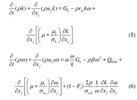
where Gkrepresents the generation of turbulent kinetic energy due to the mean velocity gradients,cµ= 0.09 and µtis the turbulent viscosity,σkand σωare the turbulent Prandtl numbers for kandω, respectively,α,β,F1and σω2are coefficients of the SSTk-ωmodel given by Egorov and Menter[13].

The difference between the SAS and SSTk-ω models is the additional term QSAS, which is associated with the von Karman length scale,LvK.

where U′andU′are the first and second velocity derivative terms, respectively,

Based on the von Karman length scale LvK, the SAS model allows to resolve the turbulence as a LES-like behavior in unsteady regions, and models the turbulence as the RANS equations in stable flow regions. The detailed description of SAS model can be found in Ref[13].

1.3 Vortex identification

The vorticity tensor is the most widely used to describe the rotational motion in a flow. But recently some research indicated that vorticity cannot distinguish between pure shearing motion and the actual rotating motion of a vortex[14]. A dimensionless quantityE is used to distinguish between the vortical, shearing and irrotational motion by Davidson[15]. This dimensionless quantityE is defined as

whereS is the strain rate andΩis vorticity tensor,

1.4 Boundary conditions

The velocity is specified at the inlet of the computational domain upstream of the patch,u=U0, and fully developed outflow is used at the outlet end of the computational domain far away from the patch, that is, with zero velocity gradient. The symmetry of boundary conditions is used at the two lateral sides and the no-slip condition is applied on the surface of cylinders.

Fig.1 Definition sketch of numerical model

1.5 Numerical procedure

The simulation is carried out by using the Fluent, a CFD software based on the finite volume approach.The Pressure Staggering Option (PRESTO) discretization scheme is used for pressure. The Bounded Central Differencing scheme is used for the momentum equations. The Quadratic Upwind Interpolation of Convective Kinematics (QUICK) algorithm is used for the turbulence equations. The Pressure Implicit with Splitting of Operators (PISO) algorithm is used for the pressure-velocity coupling.

Fig.2 Comparison between the present model and experiment[12]for mean velocity profiles,and, and root-mean- square velocityVrms

2. Model validation

The proposed numerical model is first validated by the experiments conducted by Zong and Nepf[12]to confirm the accuracy of the numerical representation of the flow development behind the circular array of cylinders. The experiments were conducted in a channel with a width of 1.2 m and a length of 13 m. The circular patch at the middle of channel was composed of emergent cylinders in a staggered arrangement. The diameter of cylinders,d , was 0.006 m. The diameter of the patch,D , was 0.22 m, with uniform flow at theinletofthechannel.Thefluidisviscousandin-

Table 1 Parameters of simulations

Fig.3 Mean velocity profiles,U and V, and root-meansquare velocityVrmsfor Cases 1-4 (φ=0.03, 0.1, 0.22 and 0.38)

compressible with the viscosity is 0.001 kg/ms–1and density is 998.2 kg/m3. The velocity was measured at the mid-depth and 3-D effects associated with the free surface and the bottom boundary were not considered in the experiments. The flow field in this study was regarded as approximately 2-D. The definition sketch of the numerical model, which is consistent with the experiment setup, is shown in Fig.1.

First, the numerical results of the case,φ=0.1 (D =0.22,U0=0.098 m/s), are compared with the experimental data of Zong and Nepf[12]for model validation. As is shown in Fig.2, the model could reproduce well(at Y =0) and(at Y= D /2) whereandare the mean velocities in the x -and ydirections, respectively. The position of the peak value of Vrms(at Y =0), the root-mean square value of the velocity in the y -direction, can also be accurately predicted, but its magnitude is over-predicted. In this case, the cylinder Reynolds number,Red= Ud/ν= 588, is greater than the typical transition value of 190 and the characteristics of flow around individual cylinders would become three-dimensional. The additional effect of 3-D turbulent vortex dissipation and vortex stretching is an important factor affecting the flow, which has not been considered in the 2-D simulation, and the bed shear friction and free surface are also ignored in the present model. These are the cause of the over-prediction of the magnitude of Vrmsin the 2-D model. Even so, the present model could capture the mean flow and main turbulence structure. The Vrmspredicted by the present model has two peaks behind the patch. The first peak occurs immediately behind the patch, corresponding to the small-scale flow generated by individual cylinders. Then the Vrmsdecreases rapidly to a small value, followed by a quick increase to the second peak as the turbulent flow develops downstream. The second peak occurs at some distance downstream the patch, corresponding to the patchscale vortices of the Karman vortex street. These results are consistent with the experimental ones of Zong and Nepf[12].

3. Numerical results

To investigate the flow pattern and drag coeffi-

cient Cd, a series of numerical simulations was conducted. The conditions of these numerical simulations are similar to the experiments of Zong and Nepf[12]. The parameters of the numerical model are summarized in Table 1.

3.1 Mean and turbulent velocity profiles

Fig.4 Streamline and concentration of the tracer (UDS)

Fig.5 Vorticity field of Cases 1-4 (φ=0.03, 0.1, 0.22 and 0.38)

3.2 Flow visualization

First, Fig.4(a) shows the streamline of Case 2. It can be seen that the flow diverges at the upstream of the patch, and becomes unsteady, propagates oscillation forward behind the patch. But regrettably, we could not see any coherent eddies structure and local flow pattern from the streamline. So a User-Defined Scalars (UDS) as a tracer material is used in the present study. The UDS equation is written as

where µt/σcis the turbulent diffusion coefficient,σcthe turbulent Schmidt number, and Scthe source term of the UDS equation. In the present study, a tracer injects into the point upstream of the patch,p(-0.6 m, 0). It means that in the UDS equation,Sc=S0in the cell of the injecting point, and in the other cells,Sc= 0. Figure 4(b) shows the concentration of the UDS for Case 2. Not only the diversion is shown, but also the coherent eddies structure could be seen in Fig.4(b). The tracer diffuses outward the central line due to the diversion and diffusion when the flow is through the patch. This tracer streak becomes unstable and yields a series of tracer eddies behind the patch. It is clearly shown that there appears the unsteady wake after the patch and the mass transport of the flow through the patch.

Fig.6 Dimensionless quantity,E , of Cases 1-4 (φ=0.03, 0.1, 0.22 and 0.38). The colours red, blue and green corresponding to E =1, -1, 0 indicate irrotational, vortical and shear motion

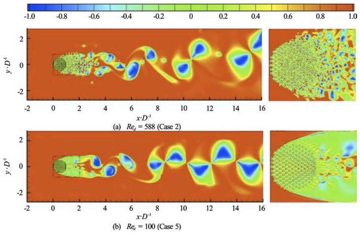
Fig.7 Dimensionless quantity E of Cases 2 and 5, with different cylinder Reynolds numbers at φ=0.1. The graphic at right is the local view of the left

3.3 Vorticity field and vortex identification

Flow around a solid body would attach and then detach from it, forming a Karman vortex street directly behind the body. Unlike the solid body case in which there is no flow through the interior of the body, when a fluid encounters a multi-body patch, one part of the fluid diverges around the patch, and the other part flows through it, forming many small-scale vortices due to individual cylinders. These small-scale vortex streets would merge or die out rapidly. The different velocities between the two parts of fluid would form a stable shear layer at the shoulder of the patch, and extend to some distance until shear instability occurs. A patch scale vortex street occurs after some distance, but not directly behind the patch, similar to that of a solid body as shown in Fig.5. The required distance to form the vortex street decreases asφincreases. For high solid volume fraction,φ=0.38, the phenomenon is very similar to that of a solid body and the classical Karman vortex street appears directly behind the patch.

In order to further analyze the flow structure in different cases, the new vortex identification characterized by the dimensionless quantityE , which was defined in Section 1.3 is used. It is shown in Fig.6 thatthe small-scale vortices in the patch are independent of each other for low solid volume fraction (φ=0.03). These small-scale vortices merge to larger-scale vortices gradually downstream. The shear layer at the shoulder of the patch is broken by the small-scale vortical motion. After some distance behind the patch, a large-patch scale Karman vortex street is formed. As φincreases, the small-scale vortices merge and die out and the length of the stable shear layer is shortened. For the case of φ=0.38, the stable shear layer does not exist at the shoulder, instead shear instability occurs and a large-scale vortical motion is observed directly behind the patch.

Fig.8 Variation of Cdwith φat Red=588

Fig.9 Variation of Cdwith Redat φ=0.1

Fig.10 Variation of Cdwith D at Red=588 and φ=0.1

Moreover, we can see that the flow at the low Reynolds number (Case 5), where Red=100 and φ= 0.1, is very different from that of the case Red=588 (Fig.7). For this low Reynolds number case, the flow is laminar and dominated by the shear motion in the patch. Practically no vortical motion exists inside and behind the patch, although the value of the solid volume fraction is moderate atφ=0.1.

Fig.11 Variation of Cdand drag force with D at the cylinder number N =144

3.4 Drag coefficient

4. Conclusions

A 2-D numerical model with SAS turbulence model has been applied to simulate the flow through a circular array of cylinders. The model is first validated by test cases where experimental data were provided by Zong and Nepf[12]. The computed results agree well with the experimental data. The numerical model based on the Fluent is capable of predicting the mean velocity profile as well as capturing the turbulence structure accurately. In order to investigate the flow

pattern and drag coefficient Cdin the flow through the circular array of cylinders, a series of numerical experiments have been carried out. For low solid volume ratio, the flow in the patch zone is dominated by the small-scale vortex street, which is generated by individual cylinders, but it would dissipate rapidly at some distance behind the patch. After this distance, the flow is dominated by the large-scale motion. For high solid volume fraction or low cylinder Reynolds number, the length of the small-scale region is shortened and the turbulent intensity in the patch zone weakened.

The drag coefficient Cdincreases with increasing φin the range of φ=0.03-0.38, but decreases with increasingRedin the range of Red=100-2000. However, the drag coefficient Cdis independent of the patch diameterDwhenφand Redare kept constant. These results are very useful reference for the estimation of the drag coefficient to be used in a porous model and for the selection of the best location for the placement of vegetation in a natural channel.

[1] GHISALBERTI M., NEPF H. M. Mixing layers and coherent structures in vegetated aquatic flow[J]. Journal of Geophysical Research, 2002, 107(C2): 1-11.

[2] NEZU I., ONITSUKA K. Turbulent structures in partly vegetated open-channel flows with LDA and PIV measurements[J]. Journal of Hydraulic Research, 2001, 39(6): 629-642.

[3] STOESSER T., SALVADOR G. P. and RODI W. et al. Large eddy simulation of turbulent flow through submerged vegetation[J]. Transport in Porous Media, 2009, 78(3): 347-365

[4] OKAMOTO T., NEZU I. Large eddy simulation of 3-D flow structure and mass transport in open-channel flows with submerged vegetations[J]. Journal of Hydro-en- vironment Research, 2010, 4(3): 185-197.

[5] SU X., LI C. W. Large eddy simulation of free surface turbulent flow in partly vegetated open channels[J]. International Journal for Numerical Methods in Fluids, 2002, 39(10): 919-937.

[6] LIU Kun, MA Dong-jun and SUN De-jun et al. Wake patterns of flow past a pair of circular cylinders in sideby-side arrangements at low Reynolds numbers[J]. Journal of Hydrodynamics, Ser. B, 2007, 19(6): 690- 697.

[7] SHARMAN B., LIEN F. S. and DAVIDSON L. et al. Numerical predictions of low Reynolds number flows over two tandem circular cylinders[J]. International Journal for Numerical Methods in Fluids, 2005, 47(5): 423-447.

[8] STONE B. M., SHEN H. T. Hydraulic resistance of flow in channels with cylindrical roughness[J]. Journal of Hydraulic Engineering, ASCE, 2002, 128(5): 500- 506.

[9] TANINO Y., NEPF H. M. Laboratory Investigation of mean drag in a random array of rigid, emergent cylinders[J]. Journal of Hydraulic Engineering, ASCE, 2008, 134(1): 34-41.

[10] TAKEMURA T., TANAKA N. Flow structures and drag characteristics of a colony-type emergent roughness model mounted on a flat plate in uniform flow[J]. Fluid Dynamics Research, 2007, 39(9-10): 694-710.

[11] NICOLLE A., EAMES I. Numerical study of flow through and around a circular array of cylinders[J]. Journal of Fluid Mechanics, 2011, 679: 1-31.

[12] ZONG L. J., NEPF H. M. Vortex development behind a finite porous obstruction in a channel[J]. Journal of Fluid Mechanics, 2012, 691: 368-391.

[13] EGOROV Y., MENTER F. Development and application of SST-SAS turbulence model in the DESIDER project[C]. Second Symposium on Hybrid RANS- LES Methods. Corfu, Greece, 2007, 261-270.

[14] VÁCLAV K. Vortex identification: New requirements and limitations[J]. International Journal of Heat and Fluid Flow, 2007, 28(4): 638-652.

[15] DAVIDSON P. A. Turbulence: An introduction for scientists and engineers[M]. Oxford, UK: Oxford University Press, 2004.

10.1016/S1001-6058(11)60371-6

* Biography: YU Ling-hui (1983-), Male, Ph. D.

ZHAN Jie-min,

E-mail:cejmzhan@gmail.com