A Jump Condition Capturing Finite Difference Schemefor Spontaneous Potential Log

LI Can-hua, PAN Ke-jia

(1.Office of Science & Technology, Hunan Normal University, Changsha 410081, China;2.School of Mathematical Science and Computing Technology, Central South University, Changsha 410075,China)

1 Introduction

The spontaneous potential(SP) log[1]plays a significant role in well log interpretation of shaly sands. It is based on the following electrochemical phenomenon. Since positive ions and negative ions have different diffusion speeds in a solution, and the grains of mud-stone often absorb positive ions,there is a steady potential difference called SP difference on any interface of different formations. These SP differences cause a spontaneous potential field in the earth. To make the corresponding log interpretation chart, it is supposed that the geometrical structure of the formation, the resistivity in each subdomain and the SP difference on each interface are all known, and the formation is symmetric about the well axis and the central plane. In figure 1, the shaded part is the area occupied by the log-tool,Ωmis the well bore filled by mud,Ωsis the enclosing rock,Ωx0is called the invasion zoneΩtis the objective layer.

Figure 1 A bounded domain with symmetric structure: H is half of the thickness of the objective formation; r0 and rx0 the radius of the well, and of the invaded zone, respectively. Here R and Z are suitably large positive constants.

In the SP log, the main feature of the formation is described by the resistivityRe>0 which is supposed to be piecewise constant, i.e.

(2)

u=E5onΓ11andu=0onΓ12,

(3)

(4)

whereΓ0is the surface of the measuring electrode composed of metallic material, the subscripts ‘+’ and ‘-’ stand for the values on both sides ofγjwhich have been prescribed in Figure 1. Conditions (6a),(6b) mean that the electric current is continuous onγj, while the potential has a jump(SP difference). Condition (5b) implies that there is no electric current emitted from the electrode.

2 Numerical Method

In this section,we introduce a new jump condition capturing finite difference method for such interface problems, which is very simple and with second order accuracy.

2.1 Difference Scheme

We suppose that the volume of the shaded part is reduced to zero, since its size is very small compared withr0, and there is no electric current emitted from it. Thus, we can solve the reduced boundary value problem on the rectangular domain[0,R]×[0,Z],andtakeuniformgridwithri= iΔr,zj= jΔz,i =0,1,…,M，j=0,1,…,N,whereΔr = R/M,Δz =Z/N.

IneachsubdomainΩi(i=1, …,4),weusestandard5-pointscheme

(7)

(a)HorizontalInterface.Assume that there is a horizontal interface (z=j0Δz), near which the resistivity isR-andR+respectively.

At horizontal interfacez=j0Δz, we employ the local Taylor expansions:

It follows that

+O(Δr+Δz).

(8)

where SUM is the sum of other four coefficients in the left side of equation (8).

(b) Vertical Interface.Assume that there is a vertical interface(r=i0Δr), near which the resistivity isR-andR+respectively. First, we rewritten(2) as

(9)

Then, we employ the local Taylor expansions at vertical interfacer=i0Δr:

(10)

(11)

From above Eqs. (9)～(11) and (6b), It follows that

(12)

where SUM is the sum of other four coeffcients in the left side of equation(12).

2.2 Error Analysis

For the sake of simplicity, we assume that the discrete scheme for the approximation solution of (2)～(6) is of the form

Lhu(P)=Fh(Γ,P),P∈Ωh,u(P)=0,P∈∂Ωh,

(13)

whereLhis finite difference “approximation” to differential operatorLin (2);Fh(Γ,P) is ‘approximations’ to the jump conditions(6).

(14)

the constantsKi, as well as the exponentsαi≥0, depending on the smoothness ofu, but independent ofh.

To prove the convergence of our method, we need the following lemma which is a straightforward generalization of Theorem 5 in[6] for elliptic interface problems.

Then the global error of the approximation solutionuhfrom (13) is bounded by

for some constantC, depending only upon the constantsKiandHi.

Theorem4Letu(r,z) be the exact solution to (2)～(6). Assumeu(r,z) has piecewisely until forth order continuous derivatives. Then we have the following error estimate for the approximation solutionuh:

Proof We take uniform grid withXi,j=(ri,zj) =(ih,jh),i=0,1,…,M,j=0,1,…,N, whereh=R/M=Z/N. Further, We assume thatr0=N1h,rx0=N2h,H=N3h, and introduce the following notations

From the derivation of method in Section 2.1, we know that the operatorLhis defined by:

It is obvious that the above difference operatorLhsatisfies the discrete maximum principle from the Theorem 3 in[6]. Sinceu(r,z) has piecewisely until forth order continuous derivatives, a simple computation leads to the following truncation error estimate:

3 Numerical Results

In this section, we examine the performance of our difference scheme for SP log interface problems. Numerical experiment shows that the scheme given in subsection 2.1 is quite accurate and effective in interpreting the log-information and in making the log interpretation chart.

To test the method, we investigate the case in which the formation has infinite radius and is homogeneous, i.e.Rm=Rx0=Rt=Rs, and some axi-symmetric double layer potentials simulating real SP differences are put in suitable positions. In this case, an “Exact” representation of SP value on the well-axis can be written as[8]

(15)

where ΔA=E3-E1-E5,ΔB=E4-E2-E3.

SettingH=2 m,r0=0.125 m,rx0=0.65 m, we compute the approximate solution by our method,and compare it with the “exact” solution given by formula(15). From Figure 2, it can be found that the approximation SP curve almost coincides with the exact SP curve for both given SP differences. Indeed in the left figure, the maximal error between the approximation SP and the exact SP on the well-axis is only 0.52 mV, the relative error is less than 0.18%.

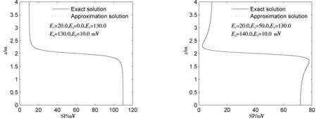
Figure 2 Comparison between approximation solutions and exact solutions

：

[1] SMITS L J. SP log interpretation in shaly sands[J]. Trans AIME, 1968, 243: 123-136.

[2] LI T T, TAN Y J, PENG Y J. Mathematical model and method for spontaneous potential well-logging[J]. European Journal of Applied Mathematics, 1994, 5: 123-139.

[3] PAN K J, TAN Y J, HU H L. Mathematical model and numerical method for spontaneous potential log in heterogeneous formations[J].Applied Mathematics and Mechanics(English Edition),2009,30(2):209-219.

[4] PENG Y J. Anecessary and suffcient condition for the well-posedness of a class of boundary value prob-lem[J]. Journal of Tongji University, 1988, 16: 91-100.

[5] ZHOU Y, CAI Z J. Convergence of a numerical method in mathematical spontaneous potential well-logging[J]. European Journal of Applied Mathematics, 1996, 7: 31-41.

[6] CIARLET P G. Discrete maximum principles for finite difference operators[J]. Aequationes Mathematica, 1970, 4: 336-352.

[7] LI H L. “Exact” solution of SP log equation in homogeneous formation[J]. Chinese Annals of Mathematics, Series A, 1996, 17: 1-8.

[8] LI T T, PENG Y J. Parameter identification in SP well-logging[J]. Inverse Problems, 2000, 16: 357-372.